Determination of Caffeine in Beverages by Spectrophotometer

Introduction: The Analytical Challenge of Quantifying Caffeine in Complex Matrices

Nowadays, milk tea, coffee, and other beverages are becoming increasingly popular worldwide. Caffeine (C8H10N4O2) is a naturally occurring purine alkaloid and the most widely consumed psychoactive substance globally. It is found in the leaves, seeds, and fruits of at least 63 plant species and is a key ingredient in coffee, tea, soft drinks, energy drinks, and many pharmaceutical formulations. Therefore, don’t assume that because you are drinking milk tea instead of coffee, it won’t affect your sleep. In fact, the caffeine content in many beverages is quite high, which can cause you to lie awake staring at the ceiling in the middle of the night. Actually, if you have a HINOTEK 752G UV Visible Spectrophotometer (priced under US$1000) and some simple solvents, you can even measure the caffeine content in your drinks at home yourself. Spectrphotoemter is a rapid, and cost-effective instrument for caffeine quantification. The instrument’s relative simplicity and the straightforward nature of the underlying principles make it a staple in academic laboratories and industrial quality assurance/quality control (QA/QC) environments.

However, the apparent simplicity of the spectrophotometric measurement belies a significant analytical challenge: the complexity of the sample matrix. Beverages are not pure solutions of caffeine. They are intricate chemical mixtures containing a wide variety of other compounds, such as sugars, natural or artificial colorants, acids, preservatives, and, in the case of coffee and tea, other structurally related alkaloids.  These co-existing substances, or “interferences,” can also absorb UV light, often in the same region as caffeine, leading to significant analytical errors. Consequently, a direct measurement of a beverage sample is almost always unviable. The true analytical challenge, therefore, lies not in the final instrumental reading but in the critical, preceding step of sample preparation. The overall accuracy, precision, and reliability of the entire method are fundamentally dictated by the efficacy of the extraction process used to isolate caffeine from its complex matrix. This article provides a comprehensive, expert-level guide to navigating this challenge, detailing the foundational principles, robust experimental protocols, and advanced considerations necessary for the accurate spectrophotometric determination of caffeine in beverages.

Section 1: Foundational Principles of Spectrophotometric Quantification

1.1 The Physics of Light Absorption: UV-Visible Spectroscopy

The ability to quantify caffeine using this method is rooted in the fundamental principles of how molecules interact with light. UV-Visible spectrophotometer measures the absorption of light in the ultraviolet (190–400 nm) and visible (325–1100 nm) regions of the electromagnetic spectrum.

Chromophores and Conjugated Systems

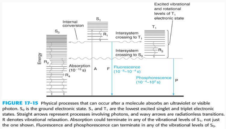
When a molecule absorbs a photon of UV or visible light, the energy from the photon promotes an electron from a lower-energy ground state orbital (S0​) to a higher-energy excited state orbital (S1​). The specific part of a molecule that is responsible for this absorption is called a chromophore.

Caffeine is an excellent chromophore because its molecular structure contains a conjugated system—a series of alternating single and double bonds. This conjugation delocalizes the

π electrons across the molecule, which lowers the energy gap between the ground and excited states. As a result, caffeine can absorb lower-energy photons, specifically in the UV range, making it readily detectable by UV-Vis spectrophotometry.

 

The Absorption Spectrum and λmax​

An absorption spectrum is a plot of a substance’s absorbance versus wavelength. For a given compound in a specific solvent, this spectrum is a unique fingerprint. The wavelength at which the maximum absorbance occurs is known as λmax​ (lambda max). Quantitative analysis is almost always performed at λmax​ for two critical reasons:

1. Maximum Sensitivity: At this wavelength, the substance absorbs light most strongly, meaning even small concentrations produce a measurable signal. This leads to lower detection limits.
2. Accuracy and Linearity: The absorbance measurement is less sensitive to small errors in wavelength calibration at the peak of a broad absorption band, ensuring better adherence to the Beer-Lambert Law.

Instrumentation Deep Dive

A UV-Vis spectrophotometer consists of several key components working in concert to produce a measurement.

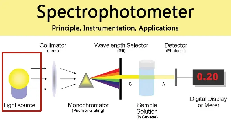
• Light Sources: To cover the full UV-Vis range, instruments typically use two lamps. A deuterium lamp provides a continuous spectrum in the UV region (typically 190–350 nm), while a tungsten-halogen lamp is used for the visible and near-infrared regions (typically 330 nm and above).
• Wavelength Selection (Monochromator): This is the heart of the spectrophotometer. Light from the source enters the monochromator through an entrance slit and is directed onto a diffraction grating. The grating disperses the light into its constituent wavelengths, much like a prism. By rotating the grating, a specific, narrow band of wavelengths can be selected to pass through an exit slit and onto the sample. The width of the exit slit controls the
  spectral bandwidth, which is a measure of the range of wavelengths passing through. A narrower bandwidth provides better spectral resolution (the ability to distinguish between two close peaks) but allows less light to reach the detector, potentially increasing signal noise.
• Sample Compartment and Cuvettes: The monochromatic light passes through the sample, which is held in a small, transparent container called a cuvette. For analysis in the UV region, cuvettes must be made of quartz, as standard glass and plastic absorb UV radiation and would interfere with the measurement.
• Detectors: After passing through the sample, the transmitted light strikes a detector, which converts the light intensity into a measurable electrical signal. Common detectors include Photomultiplier Tubes (PMTs), which are highly sensitive and stable, and silicon photodiodes, which are robust and cost-effective.
• Optical Design: Spectrophotometers can have a single-beam or double-beam design. In a single-beam instrument, the blank and the sample must be measured sequentially. A double-beam instrument splits the light beam, passing one through the sample and the other through a reference (blank) simultaneously. This design automatically corrects for fluctuations in lamp intensity over time, providing a more stable baseline and improved accuracy.

1.2 The Beer-Lambert Law: The Linchpin of Quantitative Analysis

The Beer-Lambert Law (often shortened to Beer’s Law) is the mathematical foundation that connects the amount of light absorbed by a sample to the concentration of the analyte within it. The law is expressed as: A=ϵbc
Where each term has a precise meaning :

• A (Absorbance): A dimensionless quantity representing the amount of light absorbed by the sample. It is defined on a logarithmic scale as A=log10​(I0​/I), where I0​ is the intensity of the incident light (measured using a “blank” solution containing only the solvent) and I is the intensity of the light transmitted through the sample. The logarithmic relationship is crucial because it creates a linear correlation between absorbance and concentration, which is much easier to work with than the exponential relationship of transmittance.
• ϵ (Molar Absorptivity): Also known as the molar extinction coefficient, this is a constant that is characteristic of a specific substance at a specific wavelength (λmax​). It represents how strongly the substance absorbs light. Its units are typically liters per mole-centimeter (L⋅mol−1⋅cm−1). A high molar absorptivity indicates a high probability of the electronic transition, meaning the substance is a strong absorber of light at that wavelength.
• b (Path Length): This is the distance the light travels through the sample, which is determined by the internal width of the cuvette. This is almost universally standardized to 1 cm to allow for easy comparison of results between instruments and labs.
• c (Concentration): This is the molar concentration of the absorbing substance in the solution (mol⋅L−1), which is the quantity to be determined.

The Beer-Lambert Law establishes that, for a given substance at a fixed wavelength and path length, absorbance is directly proportional to concentration. This linear relationship is what allows for the creation of a calibration curve, a graph of absorbance versus a series of known concentrations, which can then be used to determine the concentration of an unknown sample.

For more information about Spectrophotometer, please view our page:  What Is a Spectrophotometer & How Does It Work? The Ultimate Guide

Section 2: A Step-by-Step Protocol for Caffeine Analysis

This section provides a detailed, practical workflow for the quantitative determination of caffeine. Success hinges on meticulous technique, particularly in the preparation of standards and the extraction of the sample.

2.1 Preparation of Standard Solutions and Calibration Curve Construction

The calibration curve is the reference against which the unknown sample is measured. Its accuracy is therefore paramount.

Reagents and Glassware

All work must be performed using analytical grade reagents and equipment to minimize error. This includes:

• A high-purity caffeine standard (≥99%).
• Analytical grade solvents (e.g., dichloromethane, chloroform, or deionized water).
• Class A volumetric flasks and pipettes for accurate preparation of solutions.

Preparing the Stock Solution

A concentrated stock solution serves as the source for all subsequent standards.

1. Using an analytical balance to accurately weigh a precise mass of the pure caffeine standard (e.g., 100.0 mg)
2. Quantitatively transfer the solid to a volumetric flask of appropriate size (e.g., 100.0 mL).
3. Add a portion of the chosen solvent, swirl to dissolve the solid completely, and then dilute to the calibration mark with the solvent. Stopper and invert the flask several times to ensure homogeneity.
   This procedure would create a 1000 mg/L (or 1000 ppm) stock solution.

Preparing Working Standards via Serial Dilution

A series of 4 to 6 standards of decreasing concentration are prepared from the stock solution. For example, to prepare a 10 ppm standard from a 100 ppm stock solution in a 50 mL volumetric flask, one would use the dilution equation M1​V1​=M2​V2​:

(100 ppm)×V1​=(10 ppm)×(50 mL), which gives V1​=5 mL.

Thus, 5.00 mL of the stock solution would be pipetted into the 50 mL flask and diluted to the mark. This process is repeated to create a series of standards that bracket the expected concentration of the unknown sample (e.g., 2, 5, 10, 15, 20 ppm).

Determining λmax​ Experimentally

While literature often provides a λmax​ value for caffeine, this value can shift depending on the solvent and pH. A survey of methods shows reported values ranging from 260 nm to 276 nm. Blindly adopting a literature value without verifying it for the specific experimental conditions is a common but significant source of error, as it compromises sensitivity and linearity. Therefore, it is a critical best practice to determine λmax​ experimentally.

1. Select a mid-range caffeine standard (e.g., 10 ppm).
2. Using the spectrophotometer, perform a wavelength scan on this standard over the UV range (e.g., 190 nm to 350 nm), using the pure solvent as the blank.
3. The instrument software will generate a spectrum. Identify the wavelength corresponding to the highest absorbance peak. This is the experimental λmax​ that must be used for all subsequent measurements.

Generating and Validating the Calibration Curve

1. Set the spectrophotometer to the experimentally determined λmax​.
2. Zero the instrument using a cuvette filled with the pure solvent (the blank).
3. Measure the absorbance of each of the prepared working standards, starting from the least concentrated and moving to the most concentrated. Rinse the cuvette with the next standard before filling to avoid cross-contamination.
4. Plot the measured absorbance (y-axis) versus the known concentration (x-axis).
5. Perform a linear regression on the data points. The resulting output will provide the equation of the line (y=mx+b) and the coefficient of determination (R2). For a valid calibration, the
   R2 value should be very close to 1 (typically >0.995), indicating a strong linear relationship, and the y-intercept (b) should be very close to zero.

Table 1: Example Calibration Data and Linear Regression Output

This table provides a benchmark for a successful calibration using hypothetical data.

Caffeine Concentration (ppm)	Measured Absorbance at 273 nm
0 (Blank)	0.000
2.0	0.132
4.0	0.259
8.0	0.525
12.0	0.781
16.0	1.035

• Linear Regression Plot: A graph showing these points forming a straight line.
• Resulting Equation: Absorbance=0.0645×[Caffeine, ppm]+0.0021
• Coefficient of Determination: R2=0.9998

 

2.2 Sample Preparation: The Critical Extraction Step

This is the most crucial part of the analysis, designed to isolate caffeine from interfering matrix components. The choice of method depends on the sample type, available equipment, and desired throughput.

Sample Pre-treatment

• Carbonated Beverages: Must be thoroughly degassed before extraction. This can be done by stirring with a magnetic stirrer for 20 minutes, sonicating, or simply pouring the beverage back and forth between two beakers until fizzing stops. This prevents dangerous pressure buildup in the separatory funnel during extraction.
• Solid Samples (Tea/Coffee): An initial hot water extraction is needed. A known mass of tea leaves or coffee grounds is brewed in a known volume of boiling water for a set time (e.g., 20 minutes) to dissolve the caffeine into an aqueous solution, which is then filtered.

 

Method A: Liquid-Liquid Extraction (LLE)

 

LLE is a classic technique based on partitioning a solute between two immiscible liquid phases.

• Principle: Caffeine is moderately soluble in water but much more soluble in certain organic solvents like dichloromethane (CH2​Cl2​) or chloroform (CHCl3​). When the aqueous beverage sample is mixed with one of these solvents, the caffeine will preferentially move from the water phase into the organic phase. The efficiency of this transfer is described by the partition coefficient,k.
• pH Adjustment: This is a vital step for samples like tea and coffee, which contain acidic compounds called tannins. Tannins are also soluble in organic solvents and will interfere with the analysis. By adding a base such as sodium carbonate (Na2​CO3​) or sodium hydroxide (NaOH) to the aqueous sample, the tannins are deprotonated, forming ionic salts. These salts are highly soluble in water but insoluble in the organic solvent, so they remain behind in the aqueous layer while the neutral caffeine molecule is extracted.
• Procedure:

1. Place a known volume of the degassed beverage (e.g., 50 mL) into a separatory funnel.
2. Add the base (e.g., 1-2 g of Na2​CO3​ or a few mL of 1 M NaOH) and swirl to dissolve.
3. Add a portion of the organic solvent (e.g., 25 mL of CH2​Cl2​).
4. Stopper the funnel and invert it gently several times to mix the layers, venting frequently by opening the stopcock to release built-up pressure. Vigorous shaking can create an emulsion that is difficult to separate.
5. Allow the funnel to stand until the two layers have fully separated. CH2​Cl2​ and CHCl3​ are denser than water and will form the bottom layer.
6. Drain the bottom organic layer into a clean Erlenmeyer flask.
7. Repeat the extraction two more times with fresh portions of the organic solvent. Multiple extractions with smaller volumes are significantly more efficient at recovering the analyte than a single extraction with a large volume.
8. Combine all the organic extracts.

• Drying and Final Preparation: The combined organic extract may contain traces of dissolved water, which can interfere with the measurement. Add a small amount of an anhydrous drying agent, like anhydrous sodium sulfate (Na2​SO4​), and swirl until the liquid is clear. Filter or decant the dried solvent into a new flask. Gently evaporate the solvent (e.g., using a rotary evaporator or a warm water bath in a fume hood) to leave behind the crude caffeine residue. This residue is then dissolved in a precise, known volume of the analysis solvent (the same one used for the standards) for spectrophotometric measurement.

 

Method B: Solid-Phase Extraction (SPE)

SPE is a more modern and often more efficient alternative to LLE.

• Principle: SPE uses a small cartridge packed with a solid adsorbent material (the stationary phase), such as C18 silica. The sample is passed through the cartridge, and based on chemical affinity, some compounds are retained on the solid phase while others pass through. The retained compounds can then be selectively washed off with a different solvent.
• Procedure Overview:

1. Conditioning: The cartridge is prepared by passing a small volume of methanol, followed by deionized water, through it. This activates the C18 stationary phase.
2. Loading: The prepared beverage sample (often diluted) is slowly passed through the cartridge. The non-polar caffeine molecules are strongly retained by the non-polar C18 sorbent, while highly polar interferences like sugars and salts pass through to waste.
3. Washing: The cartridge is rinsed with a weak solvent (e.g., water) to wash away any remaining weakly-bound polar interferences.
4. Elution: A strong organic solvent like methanol is passed through the cartridge. This solvent disrupts the interaction between caffeine and the C18 sorbent, washing (eluting) the purified caffeine into a clean collection tube.

• Advantages: Compared to LLE, SPE is typically faster, uses significantly less solvent, is easier to automate, and often yields a cleaner extract with higher and more reproducible recovery rates.

 

2.3 Measurement and Calculation of Caffeine Content

 

Absorbance Measurement

 

The final, prepared sample extract is transferred to a quartz cuvette, and its absorbance is measured at the previously determined λmax​. It is crucial that the measured absorbance value falls within the linear range of the calibration curve. An ideal absorbance range is typically between 0.1 and 1.0. If the absorbance is too high (i.e., above the most concentrated standard), the sample solution must be accurately diluted with the solvent and re-measured. This new dilution must be accounted for in the final calculation.

 

Calculating Concentration from the Calibration Curve

 

1. Take the linear regression equation obtained from the calibration curve: y=mx+b.
2. Rearrange the equation to solve for concentration (x):
   x=my−b​
3. Substitute the measured absorbance of the unknown sample for y in the equation. The result, x, is the concentration of caffeine in the final solution that was measured in the cuvette.

Applying the Dilution Factor

This is the last critical step. The reading from the curve applies to the diluted extract, not the beverage itself. To get the original concentration, multiply the measured value by the total dilution factor.

Concentration (Original) = Concentration (Measured) × Dilution Factor

Dilution Factor = Final Volume ÷ Initial Volume

Example:

• Extract 10 mL of beverage and bring the residue back up to 50 mL.
  Dilution factor = 50 ÷ 10 = 5.
• If you then dilute that 50 mL solution 1-to-10 before testing, the overall dilution becomes 5 × 10 = 50.

Unit Conversion and Final Reporting

The concentration is often calculated in mg/L (ppm). This may need to be converted to a more consumer-friendly unit, such as mg per serving. For example, to find the amount in a 12 oz (355 mL) can:

mg per serving=Concentration (mg/L)×0.355 L/serving

Table 2: Sample Calculation for a Hypothetical Beverage
This table illustrates the complete calculation workflow.

Parameter	Value / Step
Given Data
Calibration Equation	Absorbance=0.0645×[Caffeine, ppm]+0.0021
Measured Absorbance of Sample	0.450
Initial Beverage Volume	20.0 mL
Final Extract Volume	100.0 mL
Beverage Serving Size	355 mL
Step 1: Calculate concentration in the cuvette	x=(y−b)/m x=(0.450−0.0021)/0.0645 Concentration (measured) = 6.94 ppm (or 6.94 mg/L)
Step 2: Calculate the dilution factor	Dilution Factor = Final Volume / Initial Volume Dilution Factor = 100.0 mL / 20.0 mL Dilution Factor = 5
Step 3: Calculate concentration in original beverage	Conc. (original) = Conc. (measured) × Dilution Factor Conc. (original) = 6.94 mg/L × 5 Concentration (original) = 34.7 mg/L
Step 4: Convert to mg per serving	mg/serving = Conc. (original) × Serving Volume (L) mg/serving = 34.7 mg/L × 0.355 L Final Reported Value = 12.3 mg per 355 mL serving

Section 3: Advanced Considerations: Interferences, Limitations, and Method Robustness

While the described protocol is robust, a skilled analyst must be aware of its inherent limitations and potential sources of error to generate truly reliable data.

3.1 Navigating the Chemical Maze: Potential Interferences

• Broad Matrix Effects: Even with extraction, trace amounts of highly colored compounds (like caramel color in colas) or other UV-absorbing substances can be carried over into the final extract, contributing to a positive error (an artificially high reading). This is known as a matrix effect.
• Specific Spectral Overlap: The Methylxanthine Problem: This represents the method’s primary chemical limitation, or its “Achilles’ heel.” Caffeine is part of the methylxanthine family, which also includes theobromine and theophylline. These molecules are structurally very similar to caffeine and, as a result, have similar chromophores that absorb UV light at nearly identical wavelengths.

• In beverages where caffeine is simply an additive (e.g., most colas), this is not a major issue.
• However, in products derived from natural sources like tea, coffee, and especially cocoa (used in some energy drinks and specialty coffees), theobromine and theophylline are naturally present.
• A standard liquid-liquid extraction will co-extract these related alkaloids along with caffeine. Because their absorption spectra overlap significantly with caffeine’s, the spectrophotometer cannot distinguish between them. The resulting absorbance measurement is a sum of the absorbance from all three compounds, leading to a significant overestimation of the true caffeine content. This limitation means that for complex natural products, the simple UV-Vis method is best used as a screening tool, and its results should be interpreted with caution.

3.2 Strategies for Enhancing Accuracy and Specificity

For matrices where interferences are a known problem, several advanced techniques can be employed to improve the quality of the results.

• Background Correction: A simple correction can sometimes be made by measuring the absorbance at a second wavelength where caffeine is known not to absorb, but where a constant background interference might (e.g., 310 nm or 350 nm). This background absorbance value is then subtracted from the absorbance measured at λmax​.
• Derivative Spectrophotometry: This is a powerful mathematical technique that can resolve overlapping spectral bands without physical separation. The instrument’s software calculates the first, second, or even third derivative of the absorbance spectrum (dA/dλ, d2A/dλ2, etc.). This process can amplify small differences between the spectra of caffeine and interferents, often creating “zero-crossing” points for one compound that can be used to quantify the other, or creating unique peaks and troughs for each compound that can be measured peak-to-peak. This is a key strategy for improving the accuracy of caffeine determination in complex samples like coffee and tea using only a spectrophotometer.
• Comparison with a Separatory Method (HPLC): The “gold standard” for caffeine analysis is High-Performance Liquid Chromatography (HPLC). HPLC uses a high-pressure pump to pass the sample through a column packed with a stationary phase. The components of the mixture interact differently with the column and are physically separated, eluting at different times. A detector (often a UV detector) then quantifies each component as it exits the column. Because it provides physical separation, HPLC is not susceptible to the spectral overlap issues that affect direct spectrophotometry. For research, regulatory, or product development purposes, validating the UV-Vis method against HPLC is essential to confirm its accuracy.

3.3 Understanding the Boundaries: Limitations of the Beer-Lambert Law

The linear relationship described by the Beer-Lambert Law holds true only under certain ideal conditions. Deviations from this law can lead to inaccurate results, especially if the calibration curve is extrapolated.

• Chemical Deviations: The law assumes that the absorbing molecules do not interact with each other. At high concentrations (typically >0.01 M), solute molecules can get close enough to affect each other’s electron clouds, which can slightly alter their ability to absorb light (molar absorptivity). This usually causes the calibration curve to bend downwards at high concentrations, leading to a negative deviation from linearity.
• Instrumental Deviations:
  Polychromatic Radiation: The law is strictly valid only for purely monochromatic light (light of a single wavelength). Real-world monochromators pass a narrow band of wavelengths. If the molar absorptivity of the analyte changes significantly across this band, deviations from linearity can occur. This is another reason why measuring at the flat peak of λmax​ is preferred.
  Stray Light: This refers to any extraneous light that reaches the detector without having passed through the sample correctly (e.g., from internal reflections or light leaks). Stray light becomes particularly problematic at high absorbances. As the true transmitted light (I) becomes very low, the constant stray light signal becomes a significant fraction of the total light hitting the detector, causing the measured absorbance to be artificially low. This effectively sets an upper limit on the useful absorbance range of the instrument. Double-monochromator systems are specifically designed to minimize stray light and extend the linear range.
  Physical Deviations (Scattering): If the sample solution is cloudy or contains suspended particles (e.g., from an incomplete filtration), these particles will scatter the light beam. This scattering diverts light away from the detector, which the instrument interprets as absorption, leading to a falsely high absorbance reading. All samples must be visually clear and free of particulates.

Conclusion and Recommendations

UV-Visible spectrophotometry offers a rapid, cost-effective, and powerful method for the quantification of caffeine in beverages. Its accessibility makes it an invaluable tool for educational purposes and for routine quality control in industrial settings. This article has demonstrated that while the instrumental measurement is straightforward, the method’s success is critically dependent on a well-designed and meticulously executed sample preparation protocol. The primary analytical hurdle is not the measurement of caffeine itself, but its effective isolation from a complex chemical matrix.

Based on the comprehensive analysis of the principles and potential pitfalls, the following recommendations are provided:

1. For Simple Matrices (e.g., Soft Drinks): The described liquid-liquid extraction (LLE) or solid-phase extraction (SPE) followed by direct UV-Vis measurement is a highly reliable and appropriate method. In these samples, caffeine is typically an additive, and the concentration of spectrally overlapping interferents is negligible.
2. For Complex Matrices (e.g., Tea, Coffee, Cocoa-Containing Drinks): The analyst must proceed with a heightened awareness of potential interferences, primarily from the co-extraction of other methylxanthines like theobromine and theophylline. While a standard LLE-UV-Vis protocol can provide a reasonable estimate, the results are likely to be positively biased. To improve accuracy, the use of derivative spectrophotometry is strongly recommended as it can mathematically resolve the overlapping spectra and provide a more specific quantification.
3. For Research, Method Development, and Regulatory Compliance: For applications demanding the highest degree of accuracy, specificity, and legal defensibility, the UV-Vis spectrophotometric method should be considered a screening tool. Final, reportable values must be obtained or confirmed using a validated separatory technique, with HPLC being the industry and research standard.

Ultimately, the generation of reliable analytical data requires more than just following a procedure; it demands a thorough understanding of the method’s chemistry, its inherent strengths, and its critical limitations. By applying the principles and protocols detailed in this article, analysts can confidently employ UV-Vis spectrophotometry to produce accurate and meaningful data on the caffeine content of beverages.

If you are ready to find the right UV-Vis spectrophotometer for your laboratory, please browse our complete product range:  UV-Visible Spectrophotometers

Any question, contact us by email: [email protected]

This guide is maintained by HINOTEK’s core technical team, comprised of senior engineers and application scientists with over two decades of hands-on experience in fields such as microscopy, centrifugation, and spectrophotometry. We are committed to ensuring that every piece of information in this guide—from instrument principles and technical specifications to laboratory procurement advice—maintains the highest level of accuracy and timeliness.This content is regularly reviewed and updated to reflect the latest industry standards and technological advancements. We value feedback from the global scientific community. Should you have any questions or suggestions, or wish to discuss any technical details, please do not hesitate to contact our expert team at [email protected].