What is a Fluorescence Microscope?

1. Introduction to Fluorescence Microscope 

In the landscape of modern laboratory instrumentation, the fluorescence microscope (View HINOTEK  Fluorescence Microscope Category)  stands as a cornerstone of biological and material science research. For importers, distributors, and researchers visiting HINOTEK, understanding the technical nuance of this equipment is essential not only for procurement but for ensuring the precise visualization of microscopic structures. Unlike traditional brightfield microscopy, which relies on light absorption and scattering to generate contrast, fluorescence microscopy operates on the quantum mechanical principle of fluorescence—the absorption of light at one wavelength and its subsequent emission at a longer wavelength. This capability allows for the detection of specific target molecules with extraordinary sensitivity, often against a dark background that maximizes the signal-to-noise ratio.

The fluorescence microscope has evolved from a niche instrument into a ubiquitous tool in life sciences, pathology, and materials analysis. Its ability to identify specific proteins, DNA sequences, and cellular structures within a complex matrix makes it indispensable. Whether visualizing the cytoskeleton of a cancer cell or inspecting impurities in semiconductor manufacturing, the fundamental requirement remains the same: a system capable of delivering high-intensity excitation energy while simultaneously isolating the faint emission signal with high fidelity.

This comprehensive guide serves as a definitive resource on the fluorescence microscope. We will examine the underlying photophysics, the intricate optical architecture, the diverse range of fluorophores, and the practical applications that drive scientific discovery. By mastering these concepts, laboratory managers and instrument dealers can make informed decisions regarding configuration, maintenance, and application suitability, ensuring that the chosen solution aligns perfectly with experimental demands.

2. The Physics of Fluorescence

To fully appreciate the engineering of a fluorescence microscope, one must first grasp the physical phenomena occurring at the atomic level. Fluorescence is a member of the luminescence family, distinguished specifically by the mechanism of electron excitation and the speed of emission.

2.1 Quantum Mechanics of Absorption

The process begins with the absorption of a photon. A fluorophore—a molecule capable of fluorescence—exists in a ground electronic state, typically denoted as S_0. When this molecule is exposed to light, it can absorb a photon, provided the photon’s energy matches the energy gap between the ground state and an excited state $(S_1, S_2, \dots)$. The relationship between photon energy (E) and wavelength ($\lambda$) is described by the Planck-Einstein relation:

Where:

• h is Planck’s constant $(6.626 \times 10^{-34} \text{ J}\cdot\text{s})$.
• c is the speed of light $(2.998 \times 10^8 \text{ m/s})$.
• $\nu$ is the frequency of the light.

This equation reveals that shorter wavelengths carry higher energy. Therefore, the excitation light (e.g., blue light at 488 nm) must have higher energy than the emitted light to drive the electron to the excited state.

2.2 The Jablonski Diagram and Electronic Transitions

The Jablonski diagram is the standard graphical representation used to visualize the cycle of fluorescence. It maps the energy levels of the fluorophore and the transitions electrons undergo during the fluorescence process.

1. Excitation $(10^{-15} seconds)$: The cycle initiates when an incident photon impacts the fluorophore. If the photon’s energy corresponds to the difference between the ground state ($S_0$) and an excited state ($S_1’$), an electron is promoted to a higher vibrational energy level within that excited singlet state. This transition is instantaneous on the timescale of molecular vibration, governed by the Franck-Condon principle, which states that nuclei do not move during the electronic transition.
2. Internal Conversion and Vibrational Relaxation $(10^{-14}$ to $10^{-11} seconds)$: Once in the excited state, the molecule is unstable. It rapidly dissipates excess energy through collisions with surrounding solvent molecules and internal vibration. The electron relaxes to the lowest vibrational energy level of the first excited singlet state ($S_1$). This non-radiative energy loss is a critical step; it ensures that the energy available for emission is strictly less than the energy absorbed.
3. Fluorescence Emission $(10^{-9}$ to $10^{-7} seconds)$: From the lowest vibrational level of $S_1$, the electron decays back to one of the vibrational levels of the ground state ($S_0$). This transition releases the remaining energy in the form of a photon. Because energy was lost during vibrational relaxation, the emitted photon has lower energy, lower frequency, and consequently, a longer wavelength than the absorbed photon.

2.3 The Stokes Shift

The spectral displacement between the peak of the excitation spectrum and the peak of the emission spectrum is known as the Stokes Shift, named after Sir George Gabriel Stokes who first described the phenomenon in 1852.

In the context of microscopy hardware, the Stokes Shift is the single most important characteristic of a fluorophore. It dictates the design of the optical filters. A large Stokes Shift is operationally advantageous because it allows for easy spectral separation of the intense excitation light and the weak emission signal.

• Small Stokes Shift: If the shift is small (e.g., less than 20 nm), the excitation and emission spectra overlap significantly. This makes it difficult to filter out the excitation light without also blocking a portion of the fluorescence signal, leading to images with high background noise or reduced brightness.
• Large Stokes Shift: A shift of 50 nm or greater allows for the use of wide-passband filters that capture more signal while effectively blocking the excitation source.

2.4 Quantum Yield and Fluorescence Lifetime

Two intrinsic properties determine how “bright” and “stable” a fluorophore appears under the microscope.

Quantum Yield ($\Phi$): This is the measure of emission efficiency. It represents the probability that an excited molecule will emit a photon rather than returning to the ground state via non-radiative pathways (like heat dissipation).

A quantum yield close to 1.0 (or 100%) indicates a highly efficient fluorophore, such as Fluorescein or Green Fluorescent Protein (GFP). Low quantum yield dyes require higher intensity excitation light to generate a visible signal, which can accelerate photodamage to the specimen.

Fluorescence Lifetime ($\tau$): This is the average time a molecule spends in the excited state before emitting a photon. $\tau = \frac{1}{k_f + k_{nr}}$ Where $k_f$ is the rate constant for fluorescence and $k_{nr}$ is the sum of rate constants for all non-radiative decay processes. While standard intensity-based microscopy integrates signal over time, specialized techniques like Fluorescence Lifetime Imaging Microscopy (FLIM) measure $\tau$ directly. Because $\tau$ is sensitive to the local microenvironment (pH, ion concentration, oxygen levels) but independent of dye concentration, it provides functional data that simple intensity imaging cannot.

3. Anatomy of the Fluorescence Microscope

A fluorescence microscope is a complex integration of optical, mechanical, and electronic systems. While it shares the basic stand of a conventional light microscope, its optical train is radically different. The primary engineering challenge is to deliver specific wavelengths of light to the sample and then detect the emitted fluorescence, which is often $10^3$ to $10^6$ times weaker than the excitation light. The standard configuration used today is “Epifluorescence” (incident-light fluorescence), where the objective lens serves a dual role as both the condenser and the objective.

3.1 The Light Source (Illumination System)

The light source is the engine of the fluorescence microscope. It must provide high radiance (brightness per unit area) in specific spectral bands to effectively excite the fluorophores.

3.1.1 Mercury Vapor Arc Lamps (HBO)

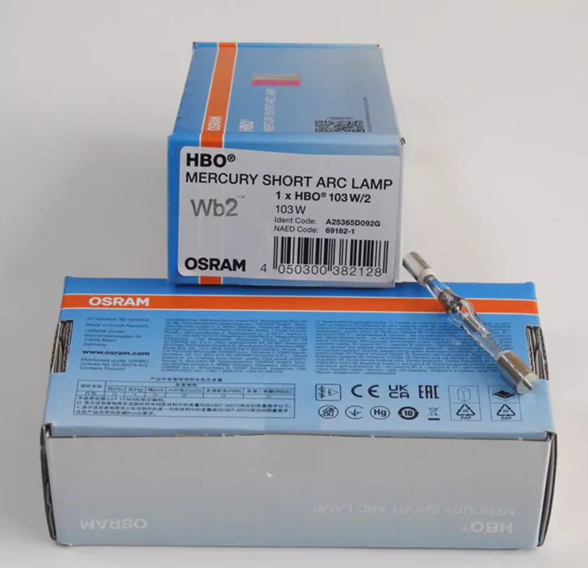For decades, the mercury arc lamp was the industry standard. These lamps contain mercury vapor under high pressure and operate by passing an electric arc between two electrodes.

• Spectral Characteristics: They produce a spectrum dominated by distinct, intense peaks (spectral lines) at specific wavelengths: 365 nm (UV), 405 nm (Violet), 436 nm (Blue), and 546 nm (Green).
• Advantages: The intensity at these specific peaks is exceptionally high, making them ideal for exciting fluorophores like DAPI (UV excitation) or Rhodamine (Green excitation).
• Disadvantages:

• Non-Uniform Spectrum: The intensity is low in the regions between the peaks, making them poor for fluorophores that require excitation at “off-peak” wavelengths (e.g., 480 nm or 630 nm).
• Lifespan: Short operational life, typically 200–300 hours.
• Safety: The bulbs contain mercury (hazardous waste) and are under high pressure, posing an explosion risk if used past their rated life. They require a warm-up period and significant alignment of the arc within the lamphouse.

3.1.2 Xenon Arc Lamps (XBO)

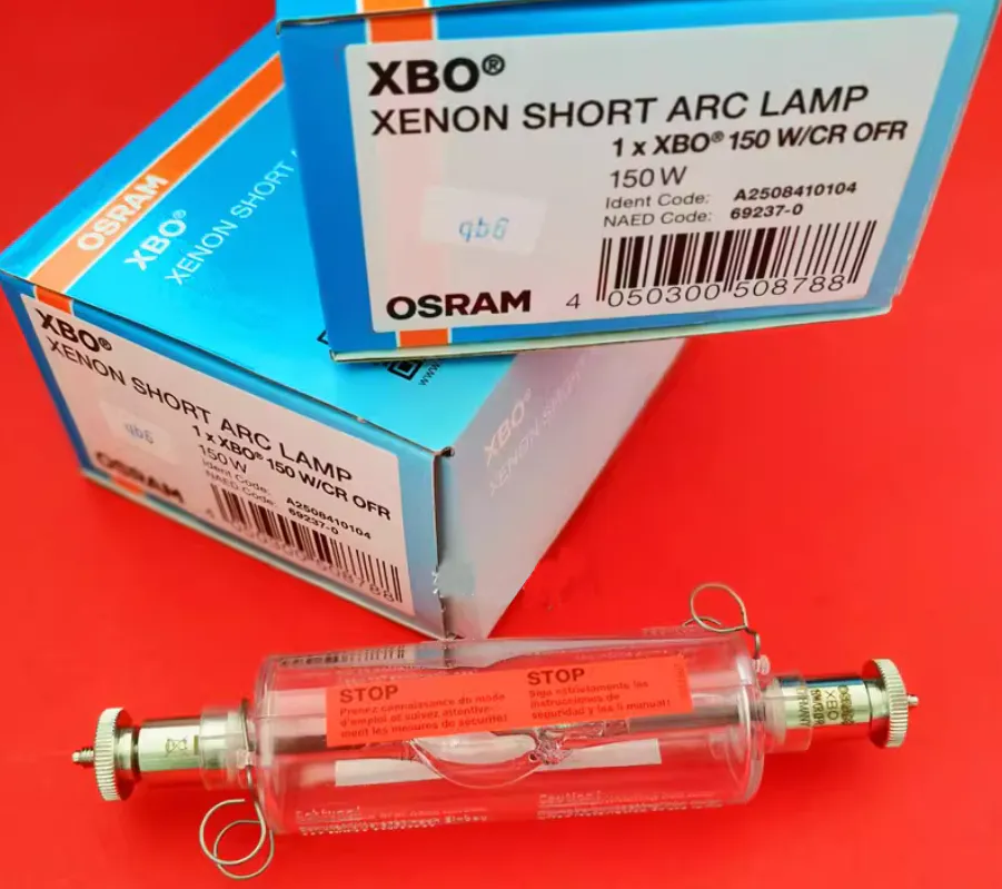• Spectral Characteristics: Xenon lamps emit a continuous spectrum that closely resembles daylight, with uniform intensity from the UV through the visible and into the infrared (IR).
• Use Cases: Because they lack the extreme peaks of mercury, they are preferred for quantitative ratiometric imaging (e.g., Fura-2 calcium imaging) where comparing intensities at different wavelengths is critical.
• Maintenance: Similar safety and alignment issues to mercury lamps, though they generally have a slightly longer lifespan.

3.1.3 Metal Halide Lamps

Metal halide systems were developed to address the shortcomings of HBO/XBO lamps.

• Design: The bulb is typically housed in a separate unit, and light is delivered to the microscope via a liquid light guide. This removes heat and vibration from the microscope frame.
• Performance: They offer a spectrum similar to mercury (with peaks) but with more continuum fill. They last much longer (approx. 2000 hours) and require no manual alignment (pre-aligned).

3.1.4 Light Emitting Diodes (LEDs)

LEDs represent the modern standard for fluorescence illumination.

• Spectral Characteristics: LEDs emit narrow, discrete bands of light (e.g., 365 nm, 470 nm, 550 nm, 635 nm). A typical LED light engine combines multiple chips to cover the UV-Visible-NIR spectrum.
• Operational Advantages:

• Longevity: Rated for 10,000 to 50,000+ hours, effectively lasting the lifetime of the microscope.
• Stability: Output is highly stable with no flicker.
• Instant Control: LEDs can be switched on and off in microseconds. This allows for electronic triggering, where the light is only on during the camera exposure time, significantly reducing photobleaching of the sample.
• Cost of Ownership: Despite a higher initial cost, the elimination of bulb replacements and lower energy consumption makes them cheaper over time.

Feature	Mercury Arc (HBO)	Xenon Arc (XBO)	Metal Halide	LED
Spectrum	Peaks (365, 436, 546)	Continuous Uniform	Peaks + Continuum	Discrete Bands
Lifespan	~200-300 hours	~400-600 hours	~2000 hours	>10,000 hours
Alignment	Critical / Difficult	Critical / Difficult	Pre-aligned	None required
Warm-up	Required (~15 min)	Required	Required	Instant On/Off
Heat	Very High	High	Moderate (Remote)	Low

3.2 The Filter Cube: The Optical Heart

The separation of excitation and emission light occurs within the fluorescence filter cube (also known as the filter block or turret). This component houses three matched optical filters.

3.2.1 Excitation Filter (Exciter)

Located in the illumination path, this filter selects the specific wavelengths from the light source that match the absorption spectrum of the fluorophore. It is typically a bandpass filter.

• Example: For GFP (Green Fluorescent Protein), an excitation filter might be a 470/40 nm bandpass, meaning it transmits light between 450 nm and 490 nm.

3.2.2 Dichroic Mirror (Beamsplitter)

This is the most sophisticated component. Positioned at a 45-degree angle at the intersection of the excitation and emission paths, it acts as a chromatic gatekeeper.

• Function: It reflects short wavelengths (excitation light) 90 degrees down through the objective to the sample. Simultaneously, it transmits longer wavelengths (fluorescence emission) returning from the sample up toward the detector.
• Mechanism: It relies on interference coatings to achieve a sharp transition edge. A dichroic for GFP might reflect light below 495 nm and transmit light above 505 nm.

3.2.3 Emission Filter (Barrier Filter)

Located in the imaging path above the dichroic, this filter blocks any residual excitation light or background scatter, passing only the fluorescence signal.

• Bandpass Emission Filters: Transmit a specific range (e.g., 525/50 nm). These are essential for multi-color imaging to prevent “bleed-through” (e.g., seeing green signal in the red channel).
• Longpass Emission Filters: Transmit all light above a certain wavelength (e.g., >520 nm). These collect more signal and are brighter, but spectral specificity is lower.

Technical Insight: Hard vs. Soft Coatings Modern HINOTEK systems utilize “hard-coated” or “sputtered” filters. Unlike older soft-coated filters which were laminated and prone to degradation from humidity and heat, hard coatings are fused to the glass substrate. They offer steeper spectral slopes (sharper transitions between blocking and transmitting) and higher transmission efficiency (>95%), resulting in brighter images with better background rejection.

3.3 The Objective Lens

In epifluorescence, the objective lens is critical because it acts as both the condenser (delivering high-intensity excitation) and the imaging lens (collecting weak emission).

3.3.1 Numerical Aperture (NA) and Brightness

The light-gathering power of an objective is defined by its Numerical Aperture: $NA = n \cdot \sin(\mu)$ Where n is the refractive index of the immersion medium and $\mu$ is the half-angle of the light cone. In fluorescence, the brightness (B) of the image is related to the fourth power of the NA: $B \propto \frac{(NA)^4}{M^2}$ This relationship implies that even a small increase in NA results in a massive increase in image brightness. For example, a 40x/1.30 oil objective collects significantly more light than a 40x/0.75 dry objective. Therefore, for fluorescence, high-NA objectives are always preferred over high magnification alone.

3.3.2 Optical Correction Classes

Objectives are categorized by their ability to correct for chromatic (color) and spherical aberrations.

• Achromat: Corrected for 2 colors (red, blue). Generally not suitable for sensitive fluorescence due to lower transmission and focus shifts between channels.
• Fluorite (Semi-Apo / FL): Corrected for 2-3 colors and spherical aberration. Constructed using fluorspar or specialized synthetic glass with high transmission in the UV/blue spectrum. These are often the “sweet spot” for fluorescence microscopy—offering excellent brightness and contrast at a reasonable cost.
• Apochromat (Plan Apo): The highest correction (4-5 colors). While they provide the sharpest resolution and flattest field, they contain many glass elements. If not specifically designed for fluorescence (e.g., Nikon “Lambda” series or Zeiss “LCI”), the extra glass can absorb some UV light or autofluoresce. However, modern Plan Apos are typically the best choice for high-end imaging.

3.3.3 Immersion Media

To achieve an NA > 1.0, immersion fluid is required to bridge the gap between the lens and cover glass, eliminating the air interface.

• Oil $(n \approx 1.515)$: Standard for high magnification. It matches the refractive index of glass. Crucial Note: Standard immersion oils can fluoresce. For fluorescence microscopy, Low Auto-Fluorescence Oil (often marked with ‘F’) must be used to prevent a hazy background.
• Water $(n \approx 1.33)$: Ideal for live-cell imaging where the sample is in aqueous media. Using oil objectives to look deep into a watery sample causes spherical aberration due to refractive index mismatch; water objectives solve this.

3.4 Detectors: The Digital Eye

While ocular observation is useful, modern analysis relies on digital sensors.

3.4.1 CCD (Charge-Coupled Device)

Traditional cooled CCDs provide excellent image quality and color fidelity. They are suitable for bright, fixed samples (e.g., histology slides). However, they are generally slower and have higher read noise than modern alternatives.

3.4.2 sCMOS (Scientific CMOS)

Scientific CMOS has largely replaced CCDs for general fluorescence.

• Characteristics: High frame rates (100 fps+), large field of view (large sensors), and extremely low read noise (< 1-2 electrons).
• Application: Ideal for live-cell imaging, high-throughput screening, and capturing fast dynamic processes.

3.4.3 EMCCD (Electron Multiplying CCD)

• Mechanism: These cameras use an on-chip gain register to amplify the electron signal before readout, effectively eliminating read noise.
• Application: Necessary only for single-molecule imaging or extreme low-light conditions where the signal is barely above the photon shot noise limit. They are expensive and generally have lower resolution (larger pixels) than sCMOS.

4. Operational Configurations

Fluorescence microscopes are available in several mechanical configurations, each suited to specific sample types.

4.1 Upright Microscope

The objective lens is positioned above the stage, and the light source directs light down onto the sample.

• Best For: Fixed slides, histology sections, and samples mounted between a slide and coverslip.
• Limitation: Not suitable for live cells in petri dishes or flasks, as the objective cannot dip into the culture media or image through the plastic lid (short working distance).

4.2 Inverted Microscope

The objective lens is positioned below the stage, looking up at the sample.

• Best For: Live-cell imaging. Cells adhere to the bottom of a petri dish or well plate. The objective images through the bottom of the vessel.
• Advantage: This leaves the top of the sample open for manipulation (e.g., micro-injection, patch-clamping) and allows the use of large culture vessels.

4.3 Stereo Fluorescence Microscope

These provide a 3D stereoscopic view at lower magnifications.

• Best For: Screening large organisms (zebrafish, Drosophila larvae), sorting transgenic colonies, or dissection under fluorescence. They often use separate optical paths for each eye to maintain depth perception.

5. Fluorophores: The Palette of Light

The success of an experiment depends heavily on selecting the right fluorophores. These probes can be broadly categorized into chemical dyes, fluorescent proteins, and quantum dots.

5.1 Organic Dyes (Fluorochromes)

These are small chemical molecules that can be conjugated to antibodies, peptides, or DNA.

• DAPI / Hoechst: DNA-binding dyes that emit blue light upon UV excitation. Used almost universally as nuclear counterstains. DAPI is generally used on fixed cells (impermeant), while Hoechst can penetrate live cells.
• Fluorescein (FITC) and Rhodamine (TRITC): The classic green and red pair. While historical, they are prone to rapid photobleaching and pH sensitivity.
• Alexa Fluor / DyLight / Cyanine (Cy): Modern synthetic dyes engineered for superior brightness, photostability, and insensitivity to pH changes. For example, Alexa Fluor 488 is a robust replacement for FITC.

5.2 Fluorescent Proteins (FPs)

Discovered in the jellyfish Aequorea victoria, Green Fluorescent Protein (GFP) revolutionized biology by allowing genetically encoded labeling.

• Mechanism: The gene for GFP is fused to the gene of a protein of interest. When the cell expresses the protein, it is inherently fluorescent.
• Palette: The family has expanded to include Blue (BFP), Cyan (CFP), Yellow (YFP), and Red (mCherry, dsRed) variants, enabling multi-color live-cell imaging.

5.3 Quantum Dots (Q-Dots)

Nanometer-scale semiconductor crystals.

• Properties: They have broad absorption spectra (can be excited by a single UV source) but very narrow, tunable emission spectra based on their size.
• Advantage: Extreme brightness and resistance to photobleaching.
• Disadvantage: Larger physical size can interfere with biological function; blinking behavior.

6. Key Applications and Protocols

The fluorescence microscope enables a diverse array of experimental techniques.

6.1 Immunofluorescence (IF)

IF uses antibodies to detect specific proteins within a cell or tissue.

• Direct IF: The primary antibody is labeled with a fluorophore. Faster but less sensitive.
• Indirect IF: A primary antibody binds the target. A secondary antibody (labeled with the fluorophore) binds the primary. This provides signal amplification (multiple secondary antibodies can bind one primary).

Protocol Overview:

1. Fixation: Treat cells with 4% Paraformaldehyde (PFA) to crosslink proteins and preserve structure.
2. Permeabilization: Use a detergent (e.g., 0.1% Triton X-100) to create pores in the cell membrane so antibodies can enter.
3. Blocking: Incubate with normal serum or BSA to block non-specific binding sites.
4. Staining: Incubate with primary antibody, wash, then incubate with secondary fluorophore-conjugated antibody.
5. Mounting: Seal with an antifade mounting medium.

6.2 Fluorescence In Situ Hybridization (FISH)

FISH detects specific DNA or RNA sequences, useful for genetic diagnostics (e.g., detecting chromosomal translocations or gene amplifications like HER2).

• Workflow: Requires “denaturing” the DNA (heating to ~75°C) to separate the double helix, allowing the fluorescent probe to hybridize to its complementary target sequence.

6.3 Live Cell Imaging

Observing dynamic processes in real-time.

• Challenges: Cells are sensitive to light (phototoxicity).
• Solution: Use minimal excitation power, highly sensitive cameras (sCMOS), and maintain physiological conditions (37°C, 5% CO2) using a stage-top incubator.

7. Maintenance and Troubleshooting

To ensure consistent performance and longevity, routine maintenance is non-negotiable.

7.1 Cleaning Protocols

Fluorescence is extremely sensitive to light loss; a dirty objective can reduce signal intensity by 50% or more.

• Frequency: Oil objectives must be cleaned immediately after every session.
• Method: Use high-quality lens tissue (never facial tissue). Moisten with a suitable solvent (70% ethanol or commercial lens cleaner). Wipe in a gentle spiral motion from the center outward to push dirt to the edge.
• Inspection: Remove the eyepiece and look down the barrel (telescope mode) to check for dust on the back focal plane of the objective.

7.2 Troubleshooting Matrix

Issue	Possible Cause	Corrective Action
No Signal / Black Image	1. Shutter closed. 2. Wrong filter cube. 3. Light source off/failed.	1. Check light path slider. 2. Match cube to dye (e.g., Blue excitation for GFP). 3. Check power supply/bulb life.
Weak / Dim Signal	1. Photobleaching. 2. Low NA objective. 3. Filter mismatch.	1. Use antifade media; reduce exposure. 2. Switch to Oil Immersion objective. 3. Verify fluorophore spectra.
High Background (Haze)	1. Autofluorescence. 2. Non-specific binding. 3. Dirty optics.	1. Use Low-Auto-Fluorescence immersion oil. 2. optimize blocking buffer concentration. 3. Clean objective and coverslip.
Uneven Illumination	1. Arc lamp misalignment. 2. Objective not centered. 3. Dirty light guide.	1. Perform lamp alignment procedure. 2. Check nosepiece seating. 3. Inspect liquid light guide for bubbles.

7.3 Photobleaching Mitigation

Photobleaching is the irreversible destruction of the fluorophore by high-intensity light.

• Strategy:

• Find Focus Quickly: Use brightfield or a dim fluorescence setting to find the sample.
• ** shuttering:** Close the fluorescence shutter whenever you are not actively acquiring an image.
• Antifade Reagents: Use mounting media containing free-radical scavengers like DABCO or n-propyl gallate.

8. Buyer’s Guide: Selecting the Right System

For HINOTEK clients, selecting a microscope involves balancing performance with budget and application requirements.

1. Define the Sample:

• Slides? Choose Upright.
• Live Cells in Dishes? Choose Inverted.
• Large Organisms? Choose Stereo.

1. Define the Fluorophores:

• Ensure the light source (LED/Lamp) and Filter Cubes match the dyes you intend to use. A standard “DAPI/FITC/TRITC” setup covers 80% of applications.

1. Camera Selection:

• Documentation? Standard Color CMOS.
• Quantification/Low Light? Monochrome sCMOS.

1. Future Proofing:

• Ensure the frame has extra ports for adding cameras or upgrade paths for motorized stages and confocal attachments.

Conclusion

The fluorescence microscope transforms the invisible world of molecular biology into a vivid, quantifiable landscape. From the quantum mechanics of the Stokes shift to the precision engineering of interference filters, every component plays a vital role in generating the final image. By adhering to rigorous maintenance schedules and optimizing optical configurations, researchers can push the limits of detection, revealing the intricate machinery of life with clarity and precision. HINOTEK remains committed to providing the advanced instrumentation required to support these scientific endeavors.

Workcite:

1. Fluorescent Microscopy – SERC (Carleton)
2. Fluorescence microscope – Wikipedia
3. Anatomy of the Fluorescence Microscope – Evident Scientific
4. Fluorescence Microscope: Principle, Parts, Uses, Examples – Microbe Notes
5. Stokes shift – Wikipedia, 
6. Fluorescence 101: A Beginners Guide to Excitation/Emission, Stokes Shift, Jablonski and More! – Bitesize Bio
7. Perrin-Jablonski Diagram – Edinburgh Instruments