A Comprehensive Guide to Fluorescence Spectrophotometer: Principles, Instrumentation, and Applications

Introduction

In the landscape of modern analytical science, few techniques unite exceptional sensitivity, high specificity, and broad applicability as effectively as fluorescence spectroscopy, also known as fluorometry or spectrofluorometry. This powerful technique has become an indispensable analytical tool in chemistry, biochemistry, and medical research, with applications extending from fundamental molecular studies to cutting-edge clinical diagnostics. At its core, the principle of fluorescence spectroscopy is deceptively simple: it involves the analysis and quantification of light emitted (fluorescence) by a sample after it has absorbed light of a specific wavelength (excitation).

However, it is this fundamental photoluminescent phenomenon that opens a window into the molecular world for scientists. By measuring the intensity, spectral characteristics (wavelength), emission polarization, and lifetime of fluorescence, researchers can obtain a wealth of information about molecular structure, dynamics, interactions, and the microenvironment in which molecules reside. The technique’s sensitivity is remarkably high, often several orders of magnitude greater than absorption spectroscopy, enabling the detection of trace substances, even down to the single-molecule level.  Furthermore, because not all molecules fluoresce, and the excitation and emission spectra of each fluorescent molecule are characteristic, the technique possesses outstanding selectivity, allowing scientists to precisely “see” target molecules within complex mixtures.

This article aims to provide laboratory managers, principal investigators, and senior scientists with a comprehensive, expert-level guide to fluorescence spectrophotometry. It will systematically elucidate the fundamental physical principles of molecular fluorescence, dissect the sophisticated architecture of modern fluorescence spectrophotometers, guide the acquisition and interpretation of various fluorescence spectral data, and showcase the transformative applications of this technology in key fields such as life sciences, environmental monitoring, and materials science. Additionally, the report will offer valuable practical guidance to help users optimize experimental design, avoid common technical pitfalls, and compare it with other spectroscopic techniques to highlight its unique value. Finally, this report will look ahead to the future trends of the technology, exploring the immense potential driven by emerging technologies like portable devices and artificial intelligence. Through this detailed report, we aim to provide a solid basis for decision-making in your laboratory’s technological investments and experimental strategies.

Section 1: Fundamental Principles of Molecular Fluorescence

To fully leverage the analytical power of fluorescence spectrophotometry, one must first gain a deep understanding of the fundamental physicochemical principles that underpin it. Fluorescence is a specific type of photoluminescence, and its unique properties make it a powerful analytical tool. This section will detail the classification of luminescent phenomena, explain the Jablonski diagram that illustrates the fluorescence process, define key photophysical parameters, and introduce the world of fluorescent molecules.

Photoluminescent Phenomena

Luminescence is a broad term for the emission of light by a substance under non-thermal conditions, hence it is also known as “cold light”. This light production can be driven by various energy sources, such as chemical reactions, electrical energy, subatomic motions, or stress on a crystal. When the excitation energy originates from photons (i.e., light), the phenomenon is called photoluminescence. Photoluminescence is primarily divided into two distinct types: fluorescence and phosphorescence. Additionally, another important form of luminescence is chemiluminescence, whose energy source is entirely different from that of photoluminescence.

• Fluorescence: This is a rapid photoluminescence process. When a molecule absorbs a photon, an electron transitions from the ground state to an excited singlet state. Within a very short time (typically nanoseconds, i.e., 10−9 to 10−6 seconds), the electron releases energy in the form of a photon and returns to the ground state. The electron transitions involved occur between energy levels of the same spin multiplicity (i.e., singlet to singlet), which is a “spin-allowed” transition, and thus happens very quickly. Fluorescence emission is almost instantaneous; once the excitation light source is turned off, the fluorescence ceases as well.
• Phosphorescence: This is a slower photoluminescence process. After a molecule is excited, its excited electron undergoes a process called “intersystem crossing,” transitioning from an excited singlet state (S₁) to an excited triplet state (T₁), which involves a reversal of the electron’s spin.Because the transition from the triplet state back to the ground singlet state (S₀) is “spin-forbidden,” its probability is much lower than that of the fluorescence process. This results in the electron remaining in the excited triplet state for a much longer time, from microseconds to seconds or even longer. Therefore, even after the excitation light source is turned off, phosphorescent materials can continue to emit light, creating an “afterglow” effect.
• Chemiluminescence: Unlike photoluminescence, the energy for chemiluminescence comes from a chemical reaction, not from the absorption of external photons.6 The chemical energy released by the reaction places the product molecules in an electronically excited state. When these molecules return to the ground state, they release energy in the form of light. Bioluminescence, such as the light from fireflies, is one of the most famous examples of chemiluminescence, driven by a chemical reaction catalyzed by an enzyme (e.g., luciferase).

The fundamental differences among these three luminescent phenomena lie in the source of excitation energy, the path of electron transition, and the timescale of light emission. Fluorescence and phosphorescence require an external light source for excitation, while chemiluminescence is driven by an intrinsic chemical reaction. The key distinction between fluorescence and phosphorescence is the spin state and lifetime of the excited state. Fluorescence involves rapid transitions between singlet states, whereas phosphorescence involves a slow transition from a long-lived triplet state to the ground state. This vast difference in timescale is not just a theoretical distinction but has practical analytical significance. For example, advanced time-resolved measurement techniques can easily distinguish between fluorescence and phosphorescence signals based on their distinctly different decay lifetimes, allowing for selective detection in complex systems.

To clearly summarize these concepts, the following table compares these three major luminescent phenomena. For laboratories planning spectroscopic analysis, a precise understanding of these terms is crucial, as they directly relate to the correct choice of instrumentation, experimental design, and data interpretation.

Table 1: Comparison of Luminescent Phenomena

Feature	Fluorescence	Phosphorescence	Chemiluminescence
Source of Excitation Energy	Photons (Light Absorption)	Photons (Light Absorption)	Chemical Reactio
Electron Transition Path	Singlet (S₁) → Singlet (S₀)	Triplet (T₁) → Singlet (S₀) (via intersystem crossing)	Excited State of Reaction Product → Ground State
Spin Conservation	Spin-Allowed (Spin multiplicity unchanged)	Spin-Forbidden (Spin multiplicity changes)	Not Applicable
Emission Timescale	Fast (nanoseconds, 10−9 – 10−6 s)	Slow (microseconds to seconds)	Duration depends on reaction rate
Requires Light Source?	Yes, emission is synchronous with excitation	Yes, but emission can persist after excitation stops (afterglow)	No, driven by the chemical reaction itself
Typical Examples	Fluorescent dyes, Tryptophan in proteins	Glow-in-the-dark materials, certain heavy metal complexes	Firefly light, Luminol reaction

 

The Jablonski Diagram: Visualizing the Fluorescence Process

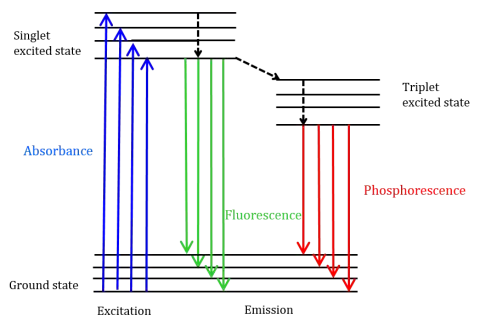
To more intuitively understand the detailed process of fluorescence, scientists use a Jablonski Diagram to describe the energy level transitions of a molecule during the absorption and emission of photons.  This diagram is the cornerstone for understanding all photophysical processes.

The fluorescence process can be broken down into the following three key steps :

1. Step 1: Excitation (Absorption)
   When a photon with appropriate energy (usually from the ultraviolet or visible region) strikes a molecule capable of fluorescence (called a fluorophore), the molecule absorbs the photon’s energy. This causes an outer electron to jump from its stable ground electronic state (S₀) to a vibrational level of a higher-energy excited singlet electronic state (usually S₁ or S₂). According to the Franck-Condon principle, this absorption process occurs very rapidly, on the order of femtoseconds (10−15 seconds), so fast that the relative positions of the molecular nuclei can be considered “frozen” during this time.
2. Step 2: Non-Radiative Relaxation
   A molecule excited to a higher vibrational level is in a highly unstable state. It rapidly loses excess energy through various non-radiative pathways to relax to lower energy levels. This process mainly includes:

• Vibrational Relaxation: Within the same electronic level, the molecule loses excess vibrational energy as heat through collisions with surrounding solvent molecules, rapidly (picoseconds, 10−12 seconds) relaxing to the lowest vibrational level of that electronic state.
• Internal Conversion: If the molecule is excited to an electronic state higher than S₁ (e.g., S₂), it typically transitions non-radiatively from S₂ to a high vibrational level of S₁, and then again reaches the lowest vibrational level of S₁ through vibrational relaxation.
  
  Both of these processes are very fast, much faster than fluorescence emission, and do not produce photons. As a result, regardless of the initial excitation wavelength (as long as the energy is sufficient), the molecule is almost always in the same, lowest-energy excited singlet state (S₁) before emitting fluorescence.
• Step 3: Fluorescence Emission
  After residing in the lowest vibrational level of S₁ for a relatively long time (the fluorescence lifetime, typically nanoseconds), the molecule finally returns to a vibrational level of the ground electronic state (S₀), emitting a photon in the process. This emitted photon is the fluorescence signal we detect. Because the molecule can relax to any of the vibrational levels of S₀, the emitted photons have a range of energies, forming an emission spectrum with a certain width rather than a single spectral line.

 

The Stokes Shift

A crucial phenomenon described by the Jablonski diagram is the Stokes Shift. It is defined as the difference between the peak wavelength of the fluorophore’s absorption spectrum (λabs​) and the peak wavelength of its emission spectrum (λem​).  Since energy is inversely proportional to wavelength (E=hc/λ), the Stokes shift essentially reflects the energy loss of the emitted photon relative to the absorbed photon.

The fundamental reason for the Stokes shift lies in the non-radiative relaxation process of the second step. Before the molecule emits fluorescence, a portion of the excitation energy has already been dissipated as heat through processes like vibrational relaxation and solvent rearrangement.  Therefore, the energy of the emitted photon (Eem​) is always lower than the energy of the absorbed photon (Eabs​), which causes the wavelength of the emitted light (λem​) to always be longer than the wavelength of the excitation light (λabs​).

This energy loss and wavelength red-shift are not mere theoretical details but are the physical basis for the ultra-high sensitivity of fluorescence technology. It is precisely because the emitted and excitation light have different wavelengths that it is possible to effectively separate them in instrument design. In a typical fluorescence spectrophotometer, the detector is placed at a 90° angle to the excitation beam.  This right-angle geometry greatly reduces the chance of intense scattered light from the excitation source (such as Rayleigh and Raman scattering) directly entering the detector. The emitted photons, due to their longer wavelength, can be further separated from the excitation photons by an emission monochromator or filter. This allows the weak fluorescence signal to be detected against a very “dark” background, thereby achieving a very high signal-to-noise ratio and detection sensitivity.  In contrast, absorption spectroscopy measures the small difference between the transmitted light passing through the sample and the incident light, both of which are high-intensity signals, making it very difficult to detect small signal changes at low concentrations.  Therefore, the Stokes shift is at the core of the huge sensitivity advantage of fluorescence spectroscopy over absorption spectroscopy.

Key Photophysical Parameters

In addition to excitation and emission wavelengths, two other key photophysical parameters are used to characterize the behavior of a fluorophore, providing valuable information about the molecule and its environment.

• Fluorescence Quantum Yield (Φ): The quantum yield is defined as the ratio of the number of photons emitted by a fluorophore to the number of photons absorbed. It measures the efficiency of the fluorescence process, with a value ranging from 0 to 1. A high quantum yield (close to 1) means that the vast majority of excited molecules return to the ground state by emitting fluorescence, making such a fluorophore very “bright.” A low quantum yield indicates that most of the energy is lost through non-radiative pathways (such as internal conversion, intersystem crossing, or collisional quenching with other molecules in the environment).  The quantum yield is very sensitive to the chemical structure of the fluorophore and its environment (e.g., solvent, temperature, pH).
• Fluorescence Lifetime (τ): The fluorescence lifetime is defined as the average time a fluorophore spends in the excited state, typically on the order of nanoseconds (10−9 s).  It is a statistical average that describes the rate at which the excited state population decays exponentially. Fluorescence lifetime is an intrinsic molecular property but is also extremely sensitive to changes in the local environment (such as the presence of quenchers, energy transfer, changes in solvent polarity, etc.). A major advantage of measuring fluorescence lifetime over fluorescence intensity is that it is an “absolute” measurement, less affected by fluorophore concentration, photobleaching, and instrumental fluctuations, thus providing more reliable information about molecular interactions and dynamic processes.

The World of Fluorophores

Molecules or parts of molecules that can produce fluorescence are called fluorophores.  Fluorophores typically contain conjugated π-electron systems, such as aromatic ring structures, which allow their electrons to absorb energy from the UV or visible region and transition to an excited state.  Fluorophores can be divided into two main categories:

• Intrinsic Fluorophores: These are naturally occurring fluorescent molecules in biological systems.  In protein research, the most important intrinsic fluorophores are the three aromatic amino acids: Tryptophan (Trp), Tyrosine (Tyr), and Phenylalanine (Phe). Among them, tryptophan has the strongest fluorescence, and its emission spectrum is most sensitive to changes in the polarity of the local environment. Therefore, by monitoring the changes in the intrinsic fluorescence of tryptophan residues in proteins, researchers can study protein conformational changes, folding/unfolding processes, and interactions with ligands without introducing external labels, making it a powerful and non-destructive analytical method.
• Extrinsic Fluorophores: These are synthetically produced fluorescent molecules, also known as fluorescent probes, dyes, or labels.  When the molecule to be analyzed does not fluoresce or has very weak fluorescence, it can be linked to an extrinsic fluorophore through covalent bonds or non-covalent interactions, allowing it to be detected by fluorescence techniques. The variety of extrinsic fluorophores is vast, including classic organic dyes (e.g., fluorescein, rhodamine, dansyl chloride), probes specifically designed to sense certain ions (like Ca²⁺) or pH, and advanced materials that have developed rapidly in recent years, such as semiconductor quantum dots (QDs).  The selectivity and diversity of these probes have greatly expanded the application range of fluorescence spectroscopy, enabling the study of almost any biological or chemical system.

Section 2: Anatomy of a Modern Fluorescence Spectrophotometer

A fluorescence spectrophotometer is a precision instrument designed for fluorescence measurements. Its goal is to efficiently deliver light of a specific wavelength to the sample and collect the emitted fluorescence with the highest sensitivity, while maximally suppressing background and noise. Understanding the construction and function of its internal components is crucial for selecting the right instrument and optimizing measurement conditions.

Core Instrument Configuration

A typical research-grade fluorescence spectrophotometer consists of core components such as a light source, an excitation monochromator, a sample compartment, an emission monochromator, and a detector. Its optical path design has a signature feature: the 90° geometry.

In a standard configuration, light from the source first passes through the excitation monochromator, which selects a specific wavelength of excitation light. This monochromatic light then illuminates the sample placed in the sample compartment. The fluorophores in the sample are excited and emit fluorescence in all directions. To minimize the detection of intense scattered excitation light, the emission monochromator and detector are placed at a 90° angle to the excitation beam. This right-angle layout is the cornerstone of fluorescence instrument design because it takes advantage of the isotropic emission of fluorescence while avoiding the transmitted and forward-scattered excitation light, thus creating a “dark background” for detecting the weak fluorescence signal, which is key to achieving a high signal-to-noise ratio.

Light Source

The function of the light source is to provide photons of sufficient intensity to effectively excite the fluorophores in the sample. An ideal light source should have high intensity, high stability, and a long lifetime over the desired wavelength range. Modern fluorescence spectrophotometers primarily use the following types of light sources:

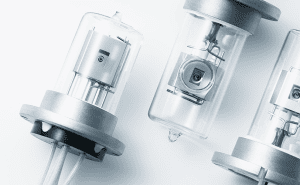
• Xenon Arc Lamps: This is the standard configuration and “workhorse” light source for the vast majority of research-grade fluorescence spectrophotometers. A xenon lamp is a high-pressure gas discharge lamp that produces a continuous, high-intensity broadband spectrum from the ultraviolet (typically >230 nm) to the near-infrared region. Its wide spectral coverage provides great flexibility, allowing users to scan and select almost any desired excitation wavelength, which is crucial for exploratory research on unknown samples or for applications requiring the measurement of excitation spectra. It is worth noting that some ozone-free xenon lamps have weaker output in the UV region below 220 nm. HINOTEK’s fluorescence spectrophotometer use Hamamatsu Xenon Arc Lamps (Life is 2000 Hours)
  

   

• Lasers: Lasers provide a highly concentrated beam of light with an extremely narrow wavelength range (excellent monochromaticity). Their extremely high irradiance makes them the preferred choice for applications requiring maximum excitation efficiency (such as single-molecule detection) or precise time control (such as time-resolved fluorescence measurements). Using a laser as a light source can eliminate the need for an excitation monochromator, but this comes at the cost of sacrificing wavelength selection flexibility, as a single laser can only provide a few fixed wavelengths.
• Light-Emitting Diodes (LEDs): In recent years, LEDs have become increasingly popular as light sources in fluorescence instruments. They offer advantages such as low cost, small size, long lifetime, and stable light output. Unlike lamps, LEDs emit a relatively narrow spectral range, making them very suitable for building dedicated, portable, or low-cost instruments for specific fluorophores. However, for general research that requires wide-range wavelength scanning, their flexibility is inferior to that of xenon lamps.

Wavelength Selection: The Role of Monochromators and Filters

Wavelength selection is the core of fluorescence measurement, determining the precise wavelengths for exciting the sample and detecting the emitted light. This function is primarily achieved by monochromators and filters.

• • Excitation and Emission Monochromators: These are the heart of a versatile fluorescence spectrophotometer, allowing the user to precisely select the excitation wavelength and scan the emission spectrum. Modern instruments almost exclusively use diffraction grating-based monochromators. Their working principle is that composite light from the source illuminates a diffraction grating, which, like a prism, disperses the light by wavelength. By precisely rotating the grating, light of a specific wavelength can be directed to an exit slit, thereby achieving monochromatic light output. A fluorescence spectrophotometer contains two independent monochromators—one for the excitation path and another for the emission path. This “dual monochromator” configuration is the fundamental difference from simpler fluorometers that use only filters and gives it great analytical flexibility, enabling it to measure excitation spectra, emission spectra, and synchronous spectra. For higher performance, some high-end instruments use double-grating monochromators (i.e., one monochromator containing two gratings), which can greatly improve stray light rejection and thus achieve a higher signal-to-noise ratio.

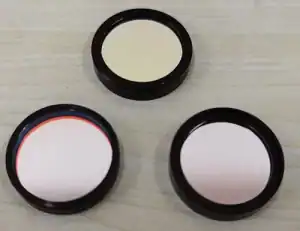
• Optical Filters: Filters are another type of wavelength selection element. They are often used to assist monochromators in further purifying the spectrum or as the primary means of wavelength selection in simpler instruments. Common types of filters include band-pass filters (which allow a specific range of wavelengths to pass), long-pass filters (which allow all light longer than a certain cutoff wavelength to pass), and short-pass filters (which allow all light shorter than a certain cutoff wavelength to pass)

Sample Compartment

The function of the sample compartment is to securely hold the sample and ensure that the light beam can pass through the sample in a predefined geometric path.

HINOTEK prodvide  many kinds of cuvettes—click here to browse them (Standard fluorescence cuvette with lid Q-203 series)

• Liquid Sample Cuvettes: These are the most common sample holders. Unlike standard absorption spectroscopy cuvettes, which have only two transparent sides, fluorescence measurement cuvettes must have at least three, and usually all four, sides optically polished. This is to accommodate the 90° detection geometry, allowing excitation light to enter from one side and emitted light to be collected from a perpendicular side.  Mixing up cuvettes is a common mistake for beginners and will lead to measurement failure. 
• Cuvette Material: The choice of material depends on the working wavelength range. For measurements in the visible region (>340 nm), ordinary optical glass cuvettes are sufficient. However, if UV region excitation or emission is involved (<340 nm), UV Quartz cuvettes must be used, as glass has strong absorption in the UV region.
• Pathlength and Volume: The standard cuvette has a pathlength (the distance the light beam travels through the sample) of 10 mm. To conserve precious samples, smaller volume semi-micro or micro cuvettes can be used.
• Other Sample Holders: To meet different application needs, modern fluorescence spectrophotometers also offer a variety of sample holders, such as those for measuring solid thin films, powders, fiber optic probes, and microplate readers for high-throughput screening.

Detector

The task of the detector is to convert the weak photon signal emitted by the sample into a measurable electrical signal. Since the fluorescence signal is often weak, the sensitivity of the detector is crucial.

• Photomultiplier Tubes (PMTs): PMTs are the most commonly used detectors in high-sensitivity fluorescence spectrophotometers. They have extremely high internal gain and can amplify a single photon event into a measurable current pulse. This “single-photon counting” capability makes them ideal for detecting extremely weak fluorescence signals, which is one of the key factors for the high sensitivity of fluorescence technology. HINOTEK’s fluorescence Spectrophotometer use PMTs.
• Other Detectors: Charge-Coupled Devices (CCD) and Complementary Metal-Oxide-Semiconductor (CMOS) detectors are multichannel detectors composed of thousands of tiny photosensitive unit arrays. They can capture the entire emission spectrum simultaneously and are often used in array spectrometers, eliminating the need to scan the emission monochromator. In recent years,
  Single-Photon Avalanche Diodes (SPADs) have gained increasing attention as a new type of high-sensitivity solid-state detector due to their excellent time resolution and photon detection efficiency in cutting-edge fields like time-resolved fluorescence and single-molecule detection.
• Monitoring Detector: Many instruments use a beam splitter to divert a small portion of the beam before it illuminates the sample, and use a monitoring detector (usually a photodiode) to monitor the intensity of the excitation source in real-time. This allows the instrument software to normalize for fluctuations in the source intensity, ensuring that the measurement results are accurate and reliable even if the source intensity drifts over time.

The instrument design itself is a system of interconnected and balanced components. For example, choosing a flexible xenon lamp source (providing a wide spectral range) necessarily requires a high-quality monochromator to achieve good spectral resolution. However, a monochromator (especially with a narrow slit setting) will significantly reduce the light flux reaching the sample. To compensate for this light loss and detect a weak signal, an extremely sensitive detector like a PMT must be used. This series of interlocking dependencies (flexibility → resolution → sensitivity) determines the final performance and cost of the instrument. Understanding this systematic trade-off helps users understand why a high-end, flexible instrument for cutting-edge research has a different configuration and price than a dedicated instrument for routine quality control, which might use only LEDs, filters, and photodiodes.

Table 2: Core Instrument Components: A Comparative Overview

Component	Common Types	Function	Advantages	Disadvantages
Light Source	Xenon Arc Lamp	Provides broadband, continuous excitation light	Wide wavelength range (UV-NIR), high flexibility, suitable for scanning excitation spectra	Limited lifetime, light intensity drifts over time, requires monitoring and correction
	Laser	Provides monochromatic, high-intensity excitation light	Extremely high brightness and monochromaticity, suitable for single-molecule, time-resolved applications	Fixed wavelength, poor flexibility, high cost
	LED	Provides excitation light in a specific band	Low cost, long lifetime, good stability, small size	Narrow wavelength range, limited flexibility, not suitable for wide-range scanning
Wavelength Selection	Diffraction Grating Monochromator	Disperses light and selects a specific wavelength	Continuously tunable, high resolution, excellent flexibility	Light flux loss, higher cost, presence of stray light
	Optical Filter	Selects a specific band of light	High light flux, low cost, simple structure	Discontinuous wavelength selection, poor flexibility
Sample Compartment	Four-sided transparent quartz cuvette	Holds liquid samples for UV-Vis measurements	Good transparency in UV-Vis region, excellent chemical inertness	High cost, fragile, requires careful cleaning
	Microplate Reader	For high-throughput sample analysis	High degree of automation, large sample throughput	Potential for inter-well interference (crosstalk), high temperature control requirements
Detector	Photomultiplier Tube (PMT)	Converts photon signals into electrical signals	Extremely high sensitivity (single-photon counting), wide dynamic range	Easily saturated, can be damaged by strong light
	CCD/CMOS Array	Captures the entire spectrum simultaneously	Fast acquisition speed (no scanning required), obtains full spectral information	Sensitivity is usually lower than PMT, higher readout noise

Section 3: Acquiring and Interpreting Fluorescence Spectra

A fluorescence spectrophotometer can provide various types of spectral data, each revealing different aspects of the sample. Mastering how to correctly acquire and interpret these spectra is key to using fluorescence technology for scientific research. This section will introduce the three most core spectral modes: emission spectra, excitation spectra, and synchronous scan spectra, as well as the more advanced three-dimensional excitation-emission matrix.

Emission Spectra

The emission spectrum is the most basic and commonly used type of spectrum in fluorescence analysis.

• Acquisition Method: First, a specific wavelength that the sample strongly absorbs is selected as the excitation wavelength (λex​) and fixed. Typically, this wavelength corresponds to a peak in the sample’s absorption spectrum. Then, by scanning the emission monochromator over a range of wavelengths longer than the excitation wavelength, the intensity of the fluorescence emitted by the sample is measured. The result is a plot of fluorescence intensity versus emission wavelength (λem​).
• Interpretation: The emission spectrum reveals the energy distribution of the photons emitted by the fluorophore as it returns to the ground state. The shape of the spectrum, its peak position (λem,max​), and its intensity are characteristic information of the fluorophore. The peak position is primarily determined by the electronic structure of the fluorophore, but it is very sensitive to changes in the local microenvironment. For example, when the polarity of the solvent around a fluorophore increases, its emission spectrum usually shifts to longer wavelengths (a red shift). The intensity of the spectrum is proportional to factors such as the concentration of the fluorophore, its quantum yield, and the intensity of the excitation light. Therefore, the emission spectrum can be used not only for qualitative identification of substances but is also the basis for quantitative analysis and the study of molecular interactions.

Excitation Spectra

The excitation spectrum provides information about the efficiency of the fluorophore in absorbing light energy.

• Acquisition Method: Contrary to the emission spectrum, to acquire an excitation spectrum, the emission monochromator is fixed at a characteristic emission peak wavelength of the sample (usually λem,max​). Then, by scanning the excitation monochromator, the sample is excited with a series of different wavelengths of light, while the fluorescence intensity at the fixed emission wavelength is recorded. The result is a plot of fluorescence intensity versus excitation wavelength (λex​).
• Interpretation: The excitation spectrum reflects the light absorption capability of the fluorophore at different wavelengths. For a pure, single-component sample, the shape of its excitation spectrum is usually identical to its UV-visible absorption spectrum. This is a very useful feature because it can be used to verify the purity of the sample—if the excitation spectrum does not match the absorption spectrum, it may indicate the presence of impurities that can transfer energy to the target fluorophore, or that the sample has undergone some chemical change. In addition, the excitation spectrum can help determine the optimal excitation wavelength, i.e., the wavelength that produces the strongest fluorescence signal, thereby achieving the highest sensitivity in subsequent quantitative experiments.

A well-known rule of thumb is the “Mirror Image Rule,” which describes that the shape of the emission spectrum of many organic fluorophores is often an approximate mirror image of its lowest energy absorption band (i.e., the long-wavelength part of the excitation spectrum). This symmetry arises from the similar spacing of the vibrational energy levels in the ground and first electronic excited states.

Synchronous Scan Spectroscopy

When a sample is a complex mixture containing multiple fluorescent components, traditional emission and excitation spectra often become blurred and difficult to resolve due to severe overlap of the spectra of the various components. Synchronous scan spectroscopy was developed to address this challenge.

• Acquisition Principle: In synchronous scan mode, the excitation and emission monochromators are scanned simultaneously, but a constant wavelength difference (Δλ=λem​−λex​) is maintained between them throughout the scan. At each excitation wavelength
  λex​, the detector only records the emission light at the wavelength λex​+Δλ.
• Types: There are mainly two modes of synchronous scanning. One is Constant-Wavelength Synchronous Luminescence (CWSL), where Δλ is kept constant. The other is Constant-Energy Synchronous Luminescence (CESL), where the energy difference (in units of wavenumbers, cm−1) between the excitation and emission light is kept constant. An advantage of CESL is that it can effectively “filter out” some spectral artifacts with a constant energy difference, such as the Raman scattering peaks of the solvent, to obtain a “cleaner” spectrum.
• Interpretation and Advantages: The main advantages of synchronous scanning are spectral simplification and increased selectivity. By carefully selecting the value of Δλ, the spectral features of a specific component can be highlighted. When the Δλ value is small (e.g., 15-20 nm), the spectrum mainly reflects the absorption characteristics of the molecule; when the Δλ value is large, the spectrum reflects more of the emission characteristics. For a mixture, by choosing a Δλ that matches the Stokes shift of the target component, its signal can be maximally enhanced while the signals of other interfering components are suppressed. This makes synchronous scanning very effective in analyzing complex systems such as polycyclic aromatic hydrocarbons (PAHs), petroleum products, and protein mixtures, enabling simultaneous qualitative and semi-quantitative analysis of different components in a mixture.

Three-Dimensional Excitation-Emission Matrices (EEMs)

Three-dimensional EEMs are one of the most powerful data acquisition modes in fluorescence spectral analysis, providing a complete fluorescence “fingerprint” of the sample.

• Acquisition Method: The acquisition of EEMs is an automated process. The instrument collects complete emission spectra at a series of continuous excitation wavelengths. By integrating all this data, a three-dimensional dataset is formed, where fluorescence intensity is a function of both excitation and emission wavelengths.  This 3D data is usually presented as a contour map, where the contour lines connect regions of the same fluorescence intensity, forming “peaks,” with each “peak” representing a fluorescent component or a class of fluorophores.
• Interpretation: EEMs provide comprehensive information about all fluorescent substances in the sample. By analyzing the position (i.e., the excitation/emission wavelength pair), shape, and intensity of the peaks in the contour map, different fluorescent components in a mixture can be identified and distinguished.  This technique is widely used in environmental science, for example, to characterize complex dissolved organic matter (DOM) in natural waters. By identifying different types of fluorescence peaks (such as humic-like peaks and protein-like peaks), the source (terrestrial or endogenous) and degradation state of the organic matter can be traced. Similarly, EEMs are used to quickly identify and characterize the source of oil spills, as different types of crude oil have their unique fluorescence fingerprints.

From simple emission/excitation spectra to synchronous scanning, and then to complex 3D EEMs, the development of fluorescence spectroscopy clearly shows the evolution of its analytical capabilities—from the initial characterization of single pure substances to the fine analysis of complex mixed systems in the real world. This evolution not only reflects the progress in instrument hardware but also drives the development of corresponding data processing methods. For example, to extract meaningful chemical information from overlapping EEM spectra, researchers have developed advanced chemometric algorithms such as Parallel Factor Analysis (PARAFAC). These algorithms can decompose complex 3D data into independent fluorescent components, thus achieving quantitative analysis of mixtures. This trend indicates that modern fluorescence spectroscopy has evolved from a mere measurement tool into an integrated analytical platform that combines advanced instrumentation, complex data acquisition modes, and powerful data analysis algorithms.

Section 4: A World of Applications

Fluorescence spectrophotometry, with its exceptional sensitivity, high selectivity, and ability to provide rich molecular information, has permeated numerous scientific research and industrial application fields. Its core value lies in its ability to translate minute molecular-level changes—whether it be a conformational shift, the breaking of a chemical bond, or environmental fluctuations—into precisely measurable optical signals. This capability allows it not only to answer “what is in the sample” but also to reveal “what is happening in the sample.”

Life Sciences and Biomedical Research

In the life sciences, fluorescence technology has become an indispensable tool, driving numerous breakthroughs from molecular biology to clinical medicine.

• Nucleic Acid and Protein Quantification: This is one of the most routine yet critically important applications of fluorescence technology. By using extrinsic dyes that specifically bind to DNA or RNA and emit strong fluorescence (such as PicoGreen for DNA quantification or RiboGreen for RNA quantification), researchers can perform high-precision quantification of nucleic acids at the nanogram or even picogram level. The sensitivity of this method is far superior to traditional methods based on UV absorption, especially when sample quantities are scarce.
• Probing Protein Structure and Conformational Changes: The function of a protein is closely related to its three-dimensional structure and dynamic changes. Fluorescence spectroscopy provides a powerful, non-destructive means to study these processes. By utilizing the protein’s own intrinsic fluorophores (mainly tryptophan residues), one can monitor in real-time the conformational changes that occur during protein folding, unfolding, ligand binding, or allosteric regulation. When the microenvironment around a tryptophan residue (e.g., polarity, accessibility) changes, its fluorescence emission spectrum’s peak position, intensity, and lifetime will change accordingly, thereby reporting on the protein’s structural dynamics. Furthermore, by introducing extrinsic fluorescent probes at specific sites on the protein, techniques like Fluorescence Resonance Energy Transfer (FRET) can be used to precisely measure intramolecular distance changes.
• High-Sensitivity Enzyme Activity Assays: The fluorescence method is one of the preferred methods for conducting enzyme kinetics studies and high-throughput drug screening. The basic strategy is to design an enzyme substrate that is quenched or non-fluorescent when intact, with a fluorescent group attached. When the enzyme catalyzes the hydrolysis of this substrate, the fluorescent group is released, and its fluorescence signal is restored or generated. By continuously monitoring the rate of increase in fluorescence intensity, the enzyme’s activity can be directly measured. The sensitivity of this method is typically several orders of magnitude higher than traditional colorimetric methods, allowing for the detection of very low concentrations of enzymes or the use of less substrate, making it ideal for high-throughput screening applications.
• Clinical Diagnostics: This is one of the most promising frontier applications of fluorescence spectroscopy. Studies have found that the autofluorescence characteristics of human tissues and body fluids change with pathological states.For example, cancerous tissues, due to their altered metabolism (such as the accumulation of endogenous fluorescent substances like porphyrins and NADH, or the degradation of structural proteins like collagen), have autofluorescence spectra that are significantly different from normal tissues.Using this characteristic, doctors can use fiber-optic probes to obtain real-time, non-invasive spectral information from tissues for auxiliary early cancer diagnosis, determining tumor margins to guide surgical resection, and monitoring treatment effects.

Environmental Science

Facing increasingly severe environmental pollution problems, fluorescence spectroscopy provides a rapid and sensitive tool for on-site or laboratory monitoring.

• Water Quality Monitoring: Dissolved organic matter (DOM) in natural water bodies is a complex mixture, and its composition and origin are important indicators for evaluating water quality and ecosystem health. Humic and protein-like substances in DOM have characteristic fluorescence signals. By acquiring 3D EEMs of water samples, a fluorescence “fingerprint” of the DOM can be obtained, allowing for rapid assessment of its origin (e.g., terrestrial input vs. biological production), degree of humification, and biodegradability. This method is also widely used to monitor the operational efficiency of wastewater treatment plants, by tracking the reduction of specific fluorescence peaks (such as peak T, associated with microbial activity) to evaluate treatment effectiveness.
• Pollutant Detection: Fluorescence spectroscopy has extremely high detection sensitivity for many environmental pollutants. Particularly for polycyclic aromatic hydrocarbons (PAHs), which are themselves strongly fluorescent, this method is a powerful tool for their trace detection. In oil spill incidents, researchers can quickly identify the type of pollution source (e.g., crude oil, diesel, or gasoline) and assess the extent of contamination by analyzing the fluorescence fingerprints of water or sediment samples. Combined with techniques like synchronous scanning, high-selectivity detection of specific pollutants can be achieved even in complex environmental matrices.

Materials Science

In the field of materials science, fluorescence spectroscopy is a core technique for characterizing the photophysical properties of luminescent materials and guiding the design of new materials.

• Characterizing Novel Luminescent Materials: For materials such as organic light-emitting diodes (OLEDs), conjugated polymers, phosphors, and rare-earth materials, fluorescence spectroscopy is used to accurately measure key parameters like their emission spectra, quantum yields, and fluorescence lifetimes. These parameters directly determine the material’s performance in applications such as displays, lighting, and sensing.
• Characterization of Quantum Dots (QDs): Quantum dots are semiconductor crystals of nanometer size, whose most significant feature is the “quantum confinement effect,” meaning their fluorescence emission wavelength can be tuned by precisely controlling their size. Fluorescence spectroscopy is the fundamental tool for characterizing quantum dots, used to determine their emission peak position, spectral width, quantum yield, and photostability.  Because quantum dots have higher quantum yields, broader absorption spectra, narrower symmetric emission peaks, and superior resistance to photobleaching compared to traditional organic dyes, they have become star materials in fields like bioimaging, high-sensitivity detection, and optoelectronic devices.

Whether it’s detecting a minute twist in a protein molecule, tracking the spread of a drop of crude oil in the vast ocean, or evaluating the luminous efficiency of a nanocrystal, the common thread in fluorescence spectroscopy is its role as a sensitive detector of “molecular events.” It not only measures the static concentration of substances but is also a powerful tool for capturing the dynamic changes of matter. This ability to translate the dynamic processes of the microscopic world into macroscopically measurable signals is the fundamental reason why fluorescence spectroscopy maintains its core position in numerous scientific fields.

Section 5: Best Practices for Robust and Reliable Measurements

Fluorescence spectroscopy is a double-edged sword. Its extreme sensitivity allows it to detect weak signals, but it also means it is highly susceptible to various interferences. Therefore, to obtain accurate and reproducible fluorescence data, a strict set of best practices must be followed, covering every aspect from experimental design to instrument parameter settings. This section provides a practical guide to help users navigate this powerful technique and avoid common analytical pitfalls.

Experimental Design and Sample Preparation

High-quality data begins with meticulous preparation. In fluorescence measurements, the sample itself is part of the optical system, and its properties directly affect the final result.

• Solvent Selection: The choice of solvent is crucial. First, high-purity solvents, such as HPLC-grade or spectroscopic-grade solvents, must be used. Common-grade solvents may contain trace amounts of aromatic impurities that produce their own fluorescence, creating a high background signal that can mask the true signal of the analyte. Second, the polarity of the solvent can significantly affect the emission spectrum of the fluorophore. Polar solvent molecules will rearrange around the excited-state fluorophore during its lifetime, leading to an increased Stokes shift (a red shift in the emission spectrum). Therefore, when comparing a series of samples, the exact same solvent system must be used to ensure the comparability of the results.
• Cuvette Selection and Handling: As mentioned earlier, fluorescence measurements must use four-sided transparent quartz cuvettes (for the UV region) or glass cuvettes (for the visible region). The cuvette must be kept absolutely clean. Fingerprints, dust, scratches, or residues from previous experiments can scatter light or produce background fluorescence. Before and after each use, it should be thoroughly rinsed with spectrally pure solvent and carefully wiped dry on the outside with a lint-free tissue. Never use brushes that can scratch the surface for cleaning.
• Concentration Management: This is the most error-prone part of fluorescence quantitative analysis. Unlike many analytical techniques, the intuition that “higher concentration means stronger signal” is wrong and even harmful in fluorescence analysis. High-concentration samples can cause a severe Inner Filter Effect (IFE), which is the main reason for quantitative failure. A widely accepted rule of thumb is:
  to ensure a good linear relationship between fluorescence intensity and concentration, the absorbance of the sample at the excitation wavelength should be kept below 0.1, preferably below 0.05. Therefore, a crucial preparatory step before fluorescence measurement is to first measure the sample’s absorption spectrum with a UV-Vis spectrophotometer and check its absorbance. If the absorbance is too high, the sample must be diluted.

Instrument Parameter Optimization

Optimizing instrument parameters is a trade-off between signal-to-noise ratio, spectral resolution, and measurement time. There is no “one-size-fits-all” set of parameters; the optimal settings depend on the specific experimental objectives.

• Slit Width (Bandpass): The slit width of the excitation and emission monochromators determines the wavelength range of the light passing through the monochromator (i.e., the spectral bandwidth or resolution) and the light flux.

• Wide Slits: Allow more light to pass through, thereby enhancing signal strength and improving the signal-to-noise ratio. The trade-off is reduced spectral resolution, meaning that closely spaced fine spectral structures cannot be resolved. Suitable for quantitative analysis of trace samples.
• Narrow Slits: Provide higher spectral resolution, allowing for clear resolution of the fine structure of the spectrum (such as vibrational peaks). However, the light flux entering the detector will decrease sharply, leading to a lower signal-to-noise ratio. Suitable for studies that require precise resolution of spectral peak shapes.
• Practical Advice: For the broad bands of most organic molecules, a medium slit width (e.g., 5 nm) is usually a good starting point. If the signal is too weak, the slit can be widened appropriately; if fine structure needs to be resolved, the slit width should be reduced.

• Scan Speed: The scan speed determines the range of wavelengths scanned by the monochromator per unit of time.

• Slow Scan: The instrument’s integration time (Dwell Time) at each data point is longer, which can average out more random noise, resulting in a smoother spectrum with a higher signal-to-noise ratio. The disadvantage is a longer measurement time.
• Fast Scan: The measurement time is short, suitable for quick overviews or kinetic studies. However, the integration time is short, and the noise level of the spectrum will be higher.
• Practical Advice: For high-quality spectra for final publication, a slower scan speed is recommended. For preliminary exploratory experiments, a fast scan can be used to save time.

• Detector Voltage (PMT Gain): For instruments using a photomultiplier tube (PMT), the high voltage (HV) applied to the PMT can be adjusted to change its gain.

• High Voltage: High gain, large signal amplification, high sensitivity. However, it also amplifies background noise, and excessive photon flux can cause PMT saturation or even damage.
• Low Voltage: Low gain, low noise, but the ability to detect weak signals is reduced.
• Practical Advice: The lowest possible voltage should be used while ensuring the signal is strong enough (typically PMT count rate > 10,000 cps). At the same time, it must be ensured that the count rate of the strongest signal is well below the PMT’s saturation limit (usually 1.5 – 2 million cps).

Avoiding Common Pitfalls

Understanding and proactively avoiding the following common spectral artifacts and interferences is key to obtaining reliable fluorescence data.

• Inner Filter Effect (IFE): This is the main source of interference in fluorescence quantitative analysis.

• Explanation: When the sample concentration is too high, the sample itself acts like a filter, affecting the propagation of light. Primary inner filter effect (pIFE) refers to the absorption of a large amount of excitation light by the sample layer close to the light source, preventing the light beam from effectively penetrating to the center of the cuvette, so that the fluorophores in the detected area are not fully excited.
  Secondary inner filter effect (sIFE) refers to the reabsorption of the fluorescence emitted from the center of the cuvette by the sample itself before it reaches the detector, which is particularly severe in molecules with a small Stokes shift. Both effects together cause the relationship between fluorescence intensity and concentration to deviate from linearity, and at high concentrations, even a “hook effect” where the signal does not increase but decreases, leading to severely underestimated quantitative results.
• Correction Strategies: The simplest and most effective method is to dilute the sample until its absorbance at the excitation wavelength is less than 0.1.Other methods include: using micro-cuvettes with a shorter path length; adopting a front-face geometry, where fluorescence is collected from the side of the sample that is excited, minimizing the path length; or using mathematical formulas (such as the Lakowicz correction formula) to correct the data post-measurement by measuring the sample’s absorption spectrum.

• Quenching: This refers to any process that causes a decrease in fluorescence intensity without involving the chemical destruction of the fluorophore. The presence of a quencher provides an additional non-radiative relaxation pathway for the excited-state molecule. Common quenchers include dissolved oxygen, halide ions, and heavy metal ions. Quenching can be
  dynamic (collision of the excited-state fluorophore with the quencher leading to energy transfer) or static (formation of a non-fluorescent complex between the fluorophore and the quencher in the ground state). In experiments, interference from potential quenchers should be eliminated or controlled.
• Photobleaching: This refers to the irreversible photochemical decomposition of a fluorophore under strong or prolonged irradiation, causing it to permanently lose its fluorescence ability. This is a particular concern in long-term observations (such as fluorescence microscopy) or when using high-intensity light sources (such as lasers). To reduce photobleaching, the lowest possible excitation light intensity should be used, exposure time should be shortened, more photostable dyes should be used, or anti-photobleaching agents should be added to the sample.

In fluorescence spectral analysis, the challenge of obtaining accurate quantitative results often lies not in the instrument measurement itself, but in a deep understanding and active control of the sample system. A novice might intuitively think that increasing the sample concentration will always yield a better signal, but the existence of the inner filter effect completely subverts this assumption. This reveals a core principle: in fluorescence measurement, the sample is not a passive object of analysis, but an active participant in the optical system. The sample’s own absorption characteristics will directly interfere with the propagation path of the excitation and emission light. Therefore, a professional analytical approach requires verifying the linear response range through serial dilution and checking the sample’s absorbance with an absorption spectrum before trusting the fluorescence data. This proactive management of the sample environment and vigilance against potential artifacts is what distinguishes reliable science from erroneous data.

Table 4: Troubleshooting Guide for Common Fluorescence Measurement Issues

Observed Problem	Possible Causes	Solutions
Signal too weak / Low S/N ratio	1. Sample concentration too low. 2. Instrument sensitivity set too low (slits too narrow, PMT voltage too low). 3. Improper excitation/emission wavelength selection.	1. Increase sample concentration appropriately. 2. Widen slits, increase PMT voltage, increase integration time or number of scan averages.	3. Measure excitation spectrum to determine the optimal excitation wavelength.
Signal exceeds detector range (saturation)	1. Sample concentration too high. 2. Instrument sensitivity set too high (slits too wide, PMT voltage too high).	1. Dilute the sample. 2. Narrow the slit width, decrease PMT voltage.
Calibration curve bends downward at high concentrations	Inner Filter Effect (IFE).	1. Preferred solution: Dilute the sample to ensure the working curve is within the linear range (A < 0.1 at excitation wavelength).	2. Use short pathlength cuvettes or front-face measurement mode.	3. Apply an absorbance correction.
Fluorescence intensity is lower than expected or decreases over time	1. Fluorescence Quenching: Presence of quenchers (e.g., O₂, Cl⁻) in the solution.	2. Photobleaching: Sample exposed to strong excitation light for a long time.	1. Check solution components; remove dissolved oxygen by bubbling with nitrogen if necessary. 2. Reduce excitation light intensity, shorten exposure time, use anti-photobleaching agents.
Unwanted sharp peaks in the spectrum	1. Rayleigh Scattering: Strong scattering peak at λem​=λex​. 2. Raman Scattering: Characteristic scattering peak from the solvent, with a fixed energy difference from the excitation light.	1. Set the starting scan wavelength of the emission spectrum 10-20 nm longer than the excitation wavelength.	2. Measure the Raman peak of the blank solvent and subtract it from the sample spectrum; or use CESL synchronous scan mode.
Poor reproducibility of results	1. Instrument instability (light source fluctuation). 2. Temperature or pH changes.	3. Inconsistent sample preparation. 4. Inconsistent cuvette placement or uncleanliness.	1. Ensure the instrument is fully warmed up; use a monitoring detector for correction. 2. Use a thermostatted sample holder and control pH with a buffer. 3. Strictly follow a standard operating procedure (SOP). 4. Ensure the cuvette is clean and placed in the same orientation for each measurement.

 

Section 6: The Broader Spectroscopic Landscape: A Comparative Analysis

To fully appreciate the unique value of fluorescence spectrophotometry, it is necessary to place it in the broader context of spectroscopic analytical techniques. By comparing it with related techniques such as UV-visible absorption spectroscopy, phosphorescence, and chemiluminescence, its advantages, limitations, and most suitable applications can be more clearly revealed.

 

Fluorescence Spectroscopy vs. UV-Visible Absorption Spectroscopy

This is one of the most important comparisons in analytical chemistry, as both techniques use UV-visible light to probe the electronic transitions of molecules. However, they have fundamental differences in their measurement principles, performance characteristics, and the information they provide.

• Sensitivity: The sensitivity of fluorescence spectroscopy is typically 1000 times higher than that of UV-visible absorption spectroscopy. This huge difference stems from their different measurement methods. Absorption spectroscopy measures the small difference between two large signals (incident light intensity
  I0​ and transmitted light intensity I), with absorbance A=log(I0​/I). When the sample concentration is very low, I is very close to I0​, and the relative error in measuring this small difference is large. In contrast, fluorescence spectroscopy directly measures the emitted photon signal on an ideal “zero background” or “dark background”. Since the excitation light has been filtered out by the 90° geometry and wavelength selection, the signal received by the detector is almost entirely from the sample, making it possible to detect extremely weak signals.
• Selectivity: Fluorescence spectroscopy has higher selectivity. First, not all molecules that absorb light will emit fluorescence, which in itself provides a layer of selectivity. Second, fluorescence analysis involves two independent wavelength parameters: excitation wavelength and emission wavelength. Even if two compounds have similar absorption spectra (excitation spectra), their emission spectra may differ significantly, allowing them to be distinguished. Absorption spectroscopy, on the other hand, relies on only one wavelength parameter. When multiple components in a mixture absorb at the same wavelength, their spectra overlap, making them difficult to distinguish.
• Information Provided: Fluorescence spectroscopy provides a much richer dimension of information than absorption spectroscopy. Absorption spectroscopy mainly provides concentration information based on the Beer-Lambert law. In addition to being used for quantitative analysis, the peak position, shape, quantum yield, and fluorescence lifetime of the emission spectrum in fluorescence spectroscopy are extremely sensitive to the local chemical environment of the fluorophore (such as polarity, pH, viscosity), molecular conformation, and dynamic processes, thus providing valuable information about molecular interactions and kinetics.
• Applicability: UV-visible absorption spectroscopy has broader applicability. Almost all molecules containing π-electrons or non-bonding electrons have absorption in the UV-visible region, making it a more universal quantitative tool. Fluorescence spectroscopy, however, is limited to molecules that can fluoresce (either intrinsically or through extrinsic labeling).

For laboratory managers, a common question is, “If I already have a UV-visible spectrophotometer, why do I need a fluorescence spectrophotometer?” The following table directly answers this question by systematically summarizing the key differences between the two techniques, clearly articulating the unique value of fluorescence in terms of sensitivity and depth of information, thereby providing a strong basis for investment decisions.

Table 3: Fluorescence Spectroscopy vs. UV-Visible Absorption Spectroscopy: A Head-to-Head Comparison

Feature	Fluorescence Spectroscopy (Fluorescence Spectrophotometer)	UV-Visible Absorption Spectroscopy (UV-Visible Spectrophotometer)
Basic Principle	Measures light emitted by a sample after absorbing light	Measures light absorbed (transmitted) by a sample
Measured Signal	Emitted photons (signal measured on a zero background)	Transmitted photons (signal is the difference between two large signals)
Sensitivity	Extremely high (can reach pM-nM levels)	Moderate (typically μM-mM levels)
Selectivity	High (depends on two wavelengths: excitation and emission)	Lower (depends on only one wavelength: absorption)
Information Provided	Quantitative, qualitative, molecular environment, conformation, dynamics, lifetime	Primarily quantitative information (concentration)
Universality	Limited (only for fluorescent or labelable molecules)	Broad (for most molecules with π-bonds or non-bonding electrons) 11
Instrument Configuration	90° detection geometry	180° linear detection geometry
Environmental Sensitivity	Very sensitive (highly affected by pH, temperature, solvent polarity)	Relatively insensitive
Primary Applications	Trace analysis, bioprobes, enzyme assays, clinical diagnostics	Routine concentration determination, OD measurements, purity analysis

 

Fluorescence vs. Phosphorescence

 

As described in Section 1, fluorescence and phosphorescence are both forms of photoluminescence, with their fundamental difference lying in the electron spin state and emission timescale.

• Electron Spin: Fluorescence is a transition from a singlet excited state (S₁) to a singlet ground state (S₀), which is spin-allowed and a fast process. Phosphorescence is a transition from a triplet excited state (T₁) to a singlet ground state (S₀), which is spin-forbidden and a slow process.
• Timescale: The lifetime of fluorescence is on the nanosecond scale, while the lifetime of phosphorescence ranges from microseconds to seconds.
  
  This huge difference in time allows for easy separation of the two using time-resolved techniques (such as with a pulsed light source). When measuring phosphorescence, a delay time can be set after the excitation pulse to allow the rapidly decaying fluorescence signal to completely disappear before the detector is turned on to collect the long-lived phosphorescence signal.

 

Fluorescence vs. Chemiluminescence

 

The difference between these two lies in the source of excitation energy.

• Fluorescence: The energy comes from the absorption of an external light source (photons), a photoluminescent process.
• Chemiluminescence: The energy comes from a chemical reaction within the system; the energy released by the reaction directly pushes the product molecules into an excited state without the need for an external light source.
  
  Although the energy sources are different, the final step of both phenomena—the emission of a photon from an excited state back to the ground state—is similar. Many fluorescence spectrophotometers can also measure chemiluminescence or bioluminescence signals by turning off the excitation source, which further increases the versatility of the instrument.

Through these comparisons, the unique position of fluorescence spectroscopy is highlighted. It far surpasses UV-visible absorption spectroscopy in sensitivity and selectivity, while providing a richer dimension of information. Compared to phosphorescence, it is more common and has a stronger signal in most biological and chemical systems. Compared to chemiluminescence, it offers better controllability, as the excitation process can be precisely controlled. These characteristics collectively determine that fluorescence spectroscopy is an irreplaceable core technology in many analytical applications that require high sensitivity and high information content.

 

Section 7: The Future of Fluorescence Spectroscopy

 

As a field that is both mature and continuously evolving, the future of fluorescence spectroscopy is filled with exciting possibilities. The driving forces of technological advancements and emerging applications are shaping the future landscape of this field. The core trend can be summarized as a shift from measuring the static “presence or absence” and “how much” to the real-time, in-situ measurement of the dynamic “what it’s doing,” “where it is,” and “how it’s changing,” reaching the ultimate precision at the single-molecule level.

 

Technological Advancements

 

Continuous innovation in instrument hardware is the fundamental driving force for the development of fluorescence technology, mainly reflected in light sources, detectors, and time-resolved techniques.

• Innovations in Light Sources and Detectors: Traditional bulky xenon lamps are being supplemented or even replaced by smaller, more stable, and more efficient light sources. The emergence of new light sources such as deep-ultraviolet LEDs (DUV-LEDs) and supercontinuum lasers provides a wider range of wavelength choices and higher brightness for excitation. On the detection side, the development of new detectors like single-photon avalanche diode (SPAD) arrays not only improves the efficiency and speed of single-photon detection but also makes it possible to integrate hundreds of detectors on a single chip, paving the way for ultra-fast, high-throughput fluorescence lifetime imaging.
• Popularization of Time-Resolved Techniques: Traditional fluorescence measurement (steady-state fluorescence) mainly focuses on fluorescence intensity and spectra, while time-resolved techniques introduce the dimension of “time” into the measurement. Techniques like Fluorescence Lifetime Imaging Microscopy (FLIM) and Fluorescence Correlation Spectroscopy (FCS) are becoming increasingly popular. FLIM generates a “functional image” that is highly sensitive to changes in the local environment (such as ion concentration, pH, molecular binding) by measuring the fluorescence lifetime at each pixel of the sample. FCS, on the other hand, obtains information such as molecular concentration, diffusion coefficient, and interaction kinetics by analyzing the fluctuations of the fluorescence signal in a tiny detection volume. These techniques allow researchers to go beyond static snapshots and observe molecular dynamic processes in living cells in real-time.

 

Emerging Trends

 

Technological advancements have given rise to new application paradigms, pushing fluorescence analysis from specialized central laboratories to broader application scenarios.

• Miniaturization and Portability: With the development of LED light sources, solid-state detectors, and miniature spectrometer technologies, the development of miniaturized, low-cost, and rugged portable fluorescence spectrometers has become an important trend. These devices liberate fluorescence analysis from the laboratory, enabling it to be used for on-site environmental monitoring (such as rapid water quality testing), on-site food safety screening, and point-of-care diagnostics in resource-limited environments.
• High-Throughput Screening (HTS): In drug discovery and genomics research, tens of thousands of samples need to be analyzed rapidly. The combination of fluorescence plate readers with automated liquid handling workstations has become a standard configuration for HTS.The high sensitivity and diverse detection modes of the fluorescence method (such as fluorescence intensity, polarization, FRET, time-resolved fluorescence) make it an ideal choice for screening compound libraries, studying protein-protein interactions, and conducting gene expression analysis.
• Single-Molecule Detection: This is the ultimate frontier of sensitivity. By confining the excitation volume to the diffraction limit (using confocal or total internal reflection microscopy) and combining it with ultra-sensitive detectors, researchers can now observe and study the behavior of single molecules. Single-molecule fluorescence technology eliminates the averaging effect of traditional ensemble measurements, revealing the heterogeneity within a molecular population and the random fluctuations of individual molecules in reaction pathways, providing an unprecedented perspective for understanding complex biological processes (such as enzyme catalysis and protein folding).
• Integration with Artificial Intelligence/Machine Learning (AI/ML): Modern fluorescence technology, especially 3D EEMs, can generate huge and complex datasets. Manual interpretation of these high-dimensional “fluorescence fingerprints” is both time-consuming and dependent on expert experience. Therefore, applying AI and machine learning algorithms to fluorescence data analysis has become a rapidly developing direction. By training neural networks, automatic classification, pattern recognition, and quantitative analysis of complex spectra can be achieved. For example, algorithms can be developed to automatically identify pollution sources based on the EEMs of water samples, or to perform automated cancer diagnosis based on tissue autofluorescence spectra, which greatly improves the efficiency and objectivity of the analysis.

The future of fluorescence spectroscopy will no longer be just an analytical chemistry tool, but a multi-dimensional biophysical and diagnostic engine. It is developing towards higher temporal resolution, spatial resolution, and sensitivity, aiming to reveal the dynamic behavior of single molecules in real-time and in-situ. In this process, the deep integration of AI/ML is not just a nice-to-have, but a necessary component for analyzing the high-dimensional complex data generated by these cutting-edge technologies, helping us to extract profound insights about the world of life and matter from massive amounts of data.

Conclusion

 

Fluorescence spectrophotometry, as a mature yet vibrant analytical science, holds an undisputed core position in modern research and industrial fields. This report has systematically elucidated the fundamental principles, instrument construction, data interpretation methods, wide-ranging applications, practical guidelines, and future trends of this technology, aiming to provide researchers and laboratory managers with a comprehensive and in-depth perspective.

The core advantages of this technique can be summarized in three keywords: unparalleled sensitivity, excellent selectivity, and rich informational dimensions. Its ability to measure weak signals against a dark background makes its sensitivity far superior to other spectroscopic techniques, enabling it to handle trace-level and even single-molecule detection tasks. The use of two wavelength parameters, excitation and emission, endows it with high selectivity for accurately identifying target substances in complex mixtures. More importantly, fluorescence spectroscopy not only answers “what is there” and “how much,” but its sensitivity to the molecular microenvironment allows it to reveal the dynamic information of “what the molecule is doing,” a capability that many other techniques cannot match.

It is these unique advantages that make the fluorescence spectrophotometer an indispensable tool in numerous fields, from basic life science research to applied materials development, from environmental quality monitoring to cutting-edge clinical diagnostics. It can be used for routine nucleic acid and protein quantification, as well as for exploring the mysteries of protein conformational changes; it can serve as a “sentinel” for environmental pollution and as a “searchlight” for early cancer diagnosis.

However, powerful capabilities also come with higher demands on the operator. To fully exploit its potential, users must have a deep understanding of the underlying photophysical principles, be vigilant and proactively avoid potential pitfalls such as the inner filter effect, quenching, and photobleaching, and ensure the accuracy and reliability of the data through careful experimental design and parameter optimization.

Looking to the future, with continuous breakthroughs in light sources, detectors, time-resolved techniques, and data analysis algorithms, fluorescence spectroscopy is developing towards higher dimensions, higher throughput, and higher intelligence. It is no longer just an instrument for measuring static data, but a powerful engine capable of providing real-time, in-situ insights into the dynamic processes of the microscopic world with single-molecule precision. For any laboratory dedicated to exploration and innovation at the molecular level, investing in and mastering fluorescence spectroscopy technology is undoubtedly a key to unlocking the door to future scientific discoveries.

This guide is maintained by HINOTEK’s core technical team, comprised of senior engineers and application scientists with over two decades of hands-on experience in fields such as microscopy, centrifugation, and spectrophotometry. We are committed to ensuring that every piece of information in this guide—from instrument principles and technical specifications to laboratory procurement advice—maintains the highest level of accuracy and timeliness.
This content is regularly reviewed and updated to reflect the latest industry standards and technological advancements. We value feedback from the global scientific community. Should you have any questions or suggestions, or wish to discuss any technical details, please do not hesitate to contact our expert team at [email protected].