An In-Depth Analysis of the Beer-Lambert Law Spectrophotometer: Theory, Application, and Limitations in Modern Spectrophotometry

Introduction

Spectrophotometry stands as a cornerstone analytical technique in the modern scientific landscape, prized for its remarkable sensitivity, versatility, and fundamentally non-destructive nature. This method, which measures the interaction of light with matter, provides invaluable quantitative and qualitative information across a vast spectrum of disciplines. At the very heart of this powerful technique lies a simple yet profound principle: the Beer-Lambert law. This law establishes the fundamental mathematical relationship that connects the physical phenomenon of light absorption to the intrinsic chemical property of concentration, thereby unlocking the potential for precise quantitative analysis.2 It is this elegant correlation that has enabled scientists to measure everything from the concentration of pollutants in our environment to the quantity of DNA in a biological sample and the purity of life-saving pharmaceuticals.

This report provides an exhaustive exploration of the Beer-Lambert law, designed to guide the reader from foundational theory to practical application and critical evaluation. The analysis will commence by establishing the physical basis of how light interacts with a chemical sample, defining the core concepts of transmittance and absorbance. It will then delve into the theoretical and historical framework of the law itself, deconstructing its components and tracing its development through the contributions of several pioneering scientists. Following this theoretical exposition, the report will examine the practical implementation of the law, detailing the instrumentation used for measurement—the spectrophotometer—and the empirical process of creating and interpreting calibration curves for quantitative analysis. The immense utility of the law will be illustrated through a multi-disciplinary survey of its applications in chemical analysis, biomedical science, environmental monitoring, and industrial quality control. Finally, the report will culminate in a nuanced and critical analysis of the law’s limitations, exploring the fundamental, chemical, and instrumental factors that define the boundaries of its applicability. Through this comprehensive journey, the Beer-Lambert law will be revealed not merely as an equation, but as a pivotal concept that continues to shape and advance scientific inquiry.

Section 1: The Fundamental Interaction of Light and Matter

1.1 The Nature of Light Absorption and Transmission

The principles of spectrophotometry are rooted in the fundamental way light interacts with matter. When a beam of electromagnetic radiation, characterized by an initial or incident intensity (I0), passes through a solution containing an absorbing substance (an analyte), its intensity is attenuated. A portion of the light is absorbed by the analyte molecules, while the remainder is transmitted through the solution with a reduced intensity (I).5 This process is not a simple mechanical blocking of light; it is a discrete, quantum-mechanical event.5

For a molecule to absorb a photon of light, the energy of that photon must precisely match the energy difference between the molecule’s stable, low-energy ground state and a higher-energy excited state. When this condition is met, the molecule absorbs the photon and is temporarily promoted to this excited electronic state.5 Because the energy levels of a molecule are quantized and unique to its structure, a given chemical species will only absorb photons of specific energies, and therefore specific wavelengths. This inherent selectivity is what gives every substance a characteristic absorption spectrum, a unique fingerprint of which wavelengths it absorbs and to what extent.

This phenomenon also explains the perceived color of a solution. The color our eyes detect is composed of the wavelengths of light that are transmitted through the solution, not absorbed. A solution appears colored because it selectively absorbs light from a particular region of the visible spectrum. The observed color is therefore the complement of the absorbed color. For instance, a solution of potassium permanganate absorbs light most strongly in the green region of the spectrum (around 525-540 nm), which is why it transmits the remaining wavelengths that combine to appear deep purple to the human eye.7 Similarly, a solution that absorbs red light will appear green.

1.2 Defining Transmittance and Absorbance

To quantify the interaction of light with a sample, two key parameters are used: transmittance and absorbance.

Transmittance (T) is formally defined as the fraction of the incident light that successfully passes through the sample and reaches the detector.9 It is a straightforward ratio of the transmitted intensity (

I) to the incident intensity (I0):T=I0I

Transmittance is a dimensionless quantity with a value ranging from 0 for a completely opaque sample that blocks all light, to for a perfectly transparent sample that transmits all light.5 In laboratory practice, it is often more convenient to express this value as a percentage, known as percent transmittance (%T):

%T=100×T=100×I0I

Absorbance (A), also commonly referred to as Optical Density (OD), is defined as the quantity of light absorbed by the solution.9 While transmittance describes how much light gets through, absorbance quantifies how much light is “stopped” by the sample. The term “Optical Density” is an older but still prevalent synonym, though its use is now officially discouraged by the International Union of Pure and Applied Chemistry (IUPAC) in favor of “absorbance”. Absorbance is also a dimensionless quantity, although it is frequently reported with “Absorbance Units” (AU), a practice that is technically redundant but common in literature.6 As will be demonstrated, absorbance is the far more useful parameter for quantitative chemical analysis because of its direct, linear relationship with the concentration of the analyte.

1.3 The Mathematical Relationship

The relationship between absorbance and transmittance is not linear but inverse and logarithmic. This mathematical connection is critical to understanding the utility of the Beer-Lambert law. Absorbance is defined as the base-10 logarithm of the reciprocal of transmittance:

A=log10(T1)=−log10(T)

By substituting the definition of transmittance (T=I/I0), we arrive at the most fundamental expression for absorbance in terms of light intensities:

A=log10(II0)

This logarithmic scale means that for each unit increase in absorbance, the amount of light transmitted through the sample decreases by a factor of ten. For example, an absorbance of 1 means that 10% of the light is transmitted, while an absorbance of 2 means that only 1% of the light is transmitted. This relationship is often a point of confusion, but it is the very reason why absorbance is the preferred metric for quantitative work. The choice is not arbitrary; it is a deliberate mathematical transformation designed to create a linear scale for analysis. The physical reality of light attenuation through a medium is an exponential decay, a relationship that is inherently non-linear and difficult to work with directly for calibration purposes. Transmittance, as a direct ratio of intensities, preserves this non-linear, exponential nature. By taking the negative logarithm of transmittance to define absorbance, this exponential curve is converted into a straight line. This linearization directly paves the way for the simple, linear form of the Beer-Lambert law, making it vastly more convenient for creating calibration curves and performing quantitative calculations.

For practical laboratory work where instruments often display percent transmittance (%T), a useful conversion formula is:

A=2−log10(%T)

The non-linear relationship between these two parameters is illustrated in Table 1, which highlights why absorbance is the superior scale for quantitative analysis. A change in absorbance from 1 to 2 represents the same absolute change as a shift from 3 to 4. However, the corresponding change in percent transmittance is drastically different (a drop from 10% to 1% versus a drop from 0.1% to 0.01%), demonstrating its non-linear nature.

Table 1: Absorbance and Transmittance Conversion

Percent Transmittance (%T)	Transmittance (T)	Absorbance (A)
100%	1.0	0.0
50%	0.5	0.301
10%	0.1	1.0
1%	0.01	2.0
0.1%	0.001	3.0
0.01%	0.0001	4.0
0.001%	0.00001	5.0
0.0001%	0.000001	6.0

Section 2: The Beer-Lambert Law: A Cornerstone of Quantitative Analysis

The Beer-Lambert law, also known as the Beer-Lambert-Bouguer law, is the central principle that underpins quantitative absorption spectroscopy. It elegantly unites the physical measurement of light absorption with the chemical property of concentration, providing a robust tool for analysis.

2.1 Historical Foundations: A Story of Scientific Accretion

The development of the Beer-Lambert law was not the work of a single individual but rather a gradual accretion of knowledge over more than a century, with each scientist building upon the work of their predecessors. This progression illustrates the evolution of a scientific principle from a broad natural observation to a precise mathematical and chemical law. The full name, Beer-Lambert-Bouguer Law, encapsulates this rich history of discovery.

Pierre Bouguer (1729): The journey began with the French mathematician and astronomer Pierre Bouguer. While studying the attenuation of starlight as it passed through the Earth’s atmosphere for his work on navigation and photometry, he made a crucial observation: the intensity of a light beam decreases in a geometric progression (i.e., exponentially) as it traverses successive layers of an absorbing medium.17 Although he correctly described this exponential relationship, he did not formulate it into the precise mathematical equation used today.19 Bouguer identified the core natural phenomenon.
Johann Heinrich Lambert (1760): Three decades later, the German physicist and mathematician Johann Heinrich Lambert cited Bouguer’s work in his own influential treatise on photometry, Photometria.17 Lambert formalized Bouguer’s observation, stating that the fraction of light absorbed by a transparent medium is independent of the incident light intensity and that each successive layer of the medium absorbs an equal fraction of the light passing through it. He isolated the physical parameter of path length and gave it a rigorous mathematical form, expressing that absorbance is directly proportional to the path length of the light through the sample (
A∝l).17
August Beer (1852): Nearly a century later, the German chemist August Beer introduced the critical chemical dimension to the law. He investigated the absorption of light by colored solutions and discovered that the absorbance of a solution is also directly proportional to the concentration of the absorbing substance (the solute).17 His contribution, establishing that
A∝c, connected the physical law of light absorption directly to the field of analytical chemistry, enabling the quantification of substances in solution.

The modern law is a synthesis of these distinct discoveries, combining the insights of all three scientists into a single, powerful relationship that links a measured optical property to both a physical dimension (path length) and a chemical property (concentration).4

2.2 Derivation of the Law

The Beer-Lambert law can be derived from a fundamental consideration of how light intensity changes as it passes through an absorbing medium. The conceptual framework begins by imagining an infinitesimally thin layer, dx, of a sample solution.

When a beam of monochromatic light with power P enters this thin layer, the decrease in its power, −dP, is directly proportional to three factors: the power of the light at that point (P), the concentration of the absorbing analyte (C), and the thickness of the layer (dx). This can be expressed as a differential equation:

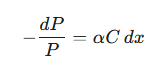where α is a proportionality constant related to the absorbing species’ ability to absorb light at that wavelength.

To find the total attenuation across the entire sample, we integrate this equation over the full path length of the light, typically the width of the cuvette, from 0 to b. The power decreases from its incident value, P0, to its transmitted value, P_T.

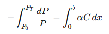Since the concentration C and the constant α are uniform throughout the homogeneous solution, they can be taken out of the integral. The integration yields:

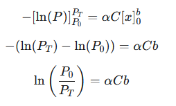This equation relates the ratio of incident to transmitted light to concentration and path length using the natural logarithm (ln). To align with the conventional definition of absorbance, which uses the base-10 logarithm, we convert the base:

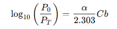Recognizing that absorbance (A) is defined as log10(P0/PT), and combining the constants α and 2.303 into a single new constant, the molar absorptivity (ϵ), we arrive at the final, familiar form of the Beer-Lambert law :

A=ϵbc

2.3 The Governing Equation: A = εbc

The most common mathematical expression of the Beer-Lambert law is:

A=ϵbc
(often written as A=ϵlc).

This equation formally states that the absorbance (A) of a solution is directly proportional to the concentration (c) of the absorbing species and the path length (b) of the light through the solution. The constant of proportionality is the molar absorptivity (ϵ). The profound utility of this equation lies in its linearity. For a given substance measured at a fixed wavelength and in a cuvette of fixed path length, ϵ and b are constants. The equation simplifies to A=(constant)×c, meaning a plot of absorbance versus concentration should yield a straight line that passes through the origin.2 This linear relationship is the bedrock of quantitative spectrophotometry.

2.4 In-Depth Analysis of Components

Each term in the Beer-Lambert equation has a precise physical meaning and specific units that are crucial for its correct application.

2.4.1 Absorbance (A)

This is the dependent variable—the quantity measured by the spectrophotometer. As established previously, it is a dimensionless value representing the logarithmic attenuation of light.

2.4.2 Path Length (b or l)

This is a controlled experimental parameter representing the distance the light travels through the sample solution.6 In practice, this is the internal width of the cuvette used to hold the sample. By international convention, the standard path length for most spectrophotometric measurements is 1 cm. This standardization simplifies calculations, as the value of b is simply 1, and facilitates the comparison of absorbance data and molar absorptivity values across different laboratories and instruments.

2.4.3 Concentration (c)

This is the independent variable, the property of the sample that is typically being determined. The law states that, all else being equal, a more concentrated solution contains more absorbing molecules in the light’s path and will therefore absorb more light than a more dilute solution.6 For the units of the equation to be consistent, concentration is typically expressed in molarity (mol/L or M).

2.4.4 Molar Absorptivity (ε)

This term, epsilon, is an intrinsic physical constant that is fundamental to the identity of the absorbing substance.

Definition: Molar absorptivity is a measure of how strongly a chemical species absorbs light at a specific wavelength. It can be thought of as a measure of the probability that a molecule will undergo an electronic transition when a photon of a particular energy strikes it. A high value of
ϵ indicates a very strong absorber at that wavelength, making the substance easy to detect even at low concentrations.
Synonyms: It is also known as the molar absorption coefficient. The older term “molar extinction coefficient” is still widely used but is discouraged by IUPAC.
Units: For the overall equation A=ϵbc to be dimensionally consistent (with A being unitless, b in cm, and c in mol/L), the units of molar absorptivity must be L mol⁻¹ cm⁻¹ (or M⁻¹ cm⁻¹).
Specificity: It is crucial to understand that ϵ is a constant only for a given substance at a specific wavelength. The value of ϵ changes as the wavelength of light changes, and this variation of ϵ with wavelength is what defines a substance’s unique absorption spectrum.
Biochemical Significance: The molar absorptivity of complex biomolecules can often be predicted from their constituent parts. For proteins, the absorbance at 280 nm is dominated by the aromatic amino acids tryptophan and tyrosine, and ϵ280 can be estimated from the protein’s amino acid sequence. Similarly, for DNA and RNA, the absorbance at 260 nm is a function of the nucleotide sequence, allowing for concentration determination without a specific standard.

To provide context for the magnitude and variability of this constant, Table 2 lists representative molar absorptivity values for several common compounds at their wavelength of maximum absorbance (λmax).

Table 2: Representative Molar Absorptivity Values

Compound	Wavelength of Max Absorbance (λmax)	Molar Absorptivity (ϵ) (L mol⁻¹ cm⁻¹)
Tryptophan	280 nm	~5,600
Tyrosine	274 nm	~1,400
Nicotinamide adenine dinucleotide (NADH)	340 nm	6,220
Potassium permanganate (KMnO4)	525 nm	~2,500
Rhodamine B	554 nm	~106,000
Values are representative and sourced from various chemical handbooks and studies, including.13

This table illustrates that ϵ is not just a theoretical factor but a measurable, characteristic property that can vary by orders of magnitude between different molecules, forming the basis for their specific and sensitive detection.

Section 3: The Spectrophotometer: The Instrument of Measurement

The Beer-Lambert law provides the theoretical framework for quantitative analysis, but its practical application relies on a sophisticated instrument known as a spectrophotometer. A spectrophotometer is engineered to precisely measure the amount of light absorbed by a sample by comparing the intensity of a light beam before and after it passes through the sample solution.11 The design of the instrument is a direct physical embodiment of the law’s requirements and assumptions, providing practical solutions to its theoretical demands.

3.1 Core Components and Functionality

A spectrophotometer is fundamentally composed of two integrated devices: a spectrometer, which produces and selects light of a specific wavelength, and a photometer, which detects and measures the light’s intensity.38 The key components are arranged sequentially to guide the light from its source to the detector.

Light Source: The process begins with a stable light source that emits a broad spectrum of radiation. The choice of lamp depends on the desired wavelength range. For measurements in the visible (approx. 400-800 nm) and near-infrared regions, a tungsten or tungsten-halogen lamp is typically used. For the ultraviolet (UV) region (approx. 200-400 nm), a deuterium lamp is required, as tungsten lamps do not emit sufficient UV radiation. Modern instruments, particularly those designed for rapid analysis, may use a xenon flash lamp, which provides high-intensity pulses of light across both the UV and visible ranges.5
Monochromator: This is arguably the most critical component, as it addresses the Beer-Lambert law’s requirement for monochromatic radiation. The monochromator takes the broadband light from the source and separates it into its constituent wavelengths. This is typically accomplished using a diffraction grating, a surface etched with thousands of precisely spaced parallel lines. When light strikes the grating, it is dispersed into a spectrum, much like a prism separates white light into a rainbow.12 The quality of the grating (e.g., modern holographic gratings versus older mechanically ruled gratings) has a direct impact on the instrument’s accuracy, particularly its ability to minimize stray light.43
Wavelength Selector (Slit): After the light is dispersed by the monochromator, an exit slit is used to physically block all wavelengths except for a very narrow band centered on the desired wavelength.38 The physical width of this slit determines the instrument’s
spectral bandwidth—the range of wavelengths that pass through to the sample. A narrower slit provides better spectral resolution and closer adherence to the monochromaticity assumption of the Beer-Lambert law, but it also reduces the total amount of light reaching the detector, which can affect signal-to-noise ratios.
Sample Compartment and Cuvettes: The selected monochromatic light then passes through the sample, which is held in the sample compartment in a specialized transparent container called a cuvette. Cuvettes are manufactured with high precision to have a fixed and known path length, which is the internal distance the light travels through the sample. The standard path length is 1 cm, a convention that satisfies the ‘b’ term in the Beer-Lambert equation and simplifies calculations.6 The material of the cuvette is also critical. For visible light measurements, inexpensive glass or plastic cuvettes are sufficient. However, for measurements in the UV range (below ~340 nm),
quartz cuvettes must be used, as both glass and plastic strongly absorb UV radiation and would interfere with the measurement.
Detector: After passing through the sample, the transmitted light (I) strikes a detector, which converts the light energy (photons) into a measurable electrical signal. The magnitude of this signal is proportional to the intensity of the light striking it. Common types of detectors include photodiodes, photodiode arrays (PDAs), and highly sensitive photomultiplier tubes (PMTs). This electrical signal is then processed by the instrument’s electronics and displayed to the user as either percent transmittance or, more commonly, absorbance.

3.2 The Light Path and Instrument Configurations

The arrangement of these components defines the light path within the spectrophotometer. A schematic representation illustrates this flow:
Light Source → Monochromator → Slit → Sample (Cuvette) → Detector → Digital Readout
This basic design can be implemented in two main configurations, each with distinct advantages and disadvantages.

Single-Beam Spectrophotometer: This is the simplest and most common design. In this configuration, the entire light beam passes through a single path to the detector. To make a measurement, the operator first inserts a “blank” cuvette into the light path. The blank contains the same solvent as the sample but lacks the analyte of interest. The instrument measures the intensity of light passing through the blank and sets this value as the 100% Transmittance or 0 Absorbance reference (I0).40 The operator then removes the blank and inserts the cuvette containing the sample. The instrument measures the new, lower intensity of transmitted light (
I) and calculates the absorbance based on the stored I0 value. While simple and cost-effective, this design is sensitive to fluctuations in the light source’s intensity that may occur in the time between measuring the blank and the sample, which can introduce error.
Double-Beam Spectrophotometer: This more advanced configuration is designed to overcome the limitations of the single-beam design. After the monochromator, a device such as a rotating mirror or beam splitter divides the light into two separate parallel beams.41 One beam—the sample beam—passes through the sample cuvette. The other beam—the reference beam—simultaneously passes through the blank cuvette.39 The instrument uses two matched detectors to measure the intensities of both beams at the same time. The electronics then compute the ratio of the two signals in real-time to determine the absorbance. This design elegantly and automatically compensates for any fluctuations in the lamp’s output, as both the sample and reference beams would be affected equally. This results in a more stable baseline and more accurate and reproducible measurements, especially for long experiments or kinetic studies.

The engineering of the spectrophotometer is a testament to the symbiotic relationship between physical theory and analytical hardware. Each key component directly addresses a requirement or a potential vulnerability of the Beer-Lambert law. The monochromator and slit provide the monochromatic radiation assumed by the law. The precisely manufactured cuvette provides the defined path length. The procedure of measuring a blank establishes the reference intensity, I0. Finally, the sophisticated double-beam design is an elegant engineering solution to nullify the potential instrumental error caused by light source instability. Thus, the instrument itself is a physical manifestation of the principles it is designed to measure.

Section 4: Practical Application: From Theory to Measurement

While the Beer-Lambert equation, A=ϵbc, provides the theoretical foundation for quantitative spectrophotometry, the most robust and common method for determining the concentration of an unknown sample in practice is through the use of a calibration curve. This empirical approach establishes the precise relationship between absorbance and concentration under the specific experimental conditions, including the particular instrument, solvent, and temperature, thereby accounting for minor, real-world deviations from ideal behavior.

4.1 The Calibration Curve: The Empirical Application of the Law

A calibration curve, also known as a standard curve, is a graph that plots the measured absorbance versus the known concentration of a series of standard solutions.47 The purpose of this curve is to create a reliable model that can be used to accurately predict the concentration of an unknown sample by simply measuring its absorbance.46 By preparing a set of standards that bracket the expected concentration of the unknown, the analyst can empirically verify the linear relationship predicted by the Beer-Lambert law within that specific range and use the resulting best-fit line for interpolation.

4.2 Step-by-Step Guide to Creating a Calibration Curve

The construction of a valid calibration curve requires careful planning and precise laboratory technique.

Step 1: Preparation of a Stock Solution: The process begins with the preparation of a single, concentrated stock solution from which all other standards will be made. This is typically done by accurately weighing a known mass of a pure, solid standard and dissolving it in a specific volume of the chosen solvent using a volumetric flask to ensure high accuracy.46 The purity of the standard and the precision of the weighing and volume measurements are critical, as any error in the stock solution will propagate through all subsequent dilutions.
Step 2: Preparation of Standard Solutions via Serial Dilution: The concentrated stock solution is then used to create a series of more dilute standard solutions. A common method for this is serial dilution, where a specific volume of the stock solution is diluted to create the first standard, then the same volume of that first standard is diluted to create the second, and so on.46 This creates a series of standards (a minimum of five is recommended for a reliable curve) with decreasing concentrations that span the desired analytical range.46 While serial dilution is common, it is worth noting that any pipetting error in one step will be carried over to all subsequent standards. The ideal, though more labor-intensive, method is to prepare each standard independently from the stock solution to avoid this propagation of error.49 Precision in pipetting and the use of clean, calibrated volumetric glassware are paramount in this step.
Step 3: Spectrophotometer Setup and Measurement:

Wavelength Selection: The spectrophotometer must be set to the optimal wavelength for the analysis. This is almost always the wavelength of maximum absorbance (λmax) for the analyte, which can be determined by scanning the absorption spectrum of one of the standards. Measuring at λmax provides two key advantages: it offers the greatest sensitivity (the largest change in absorbance for a given change in concentration), and it minimizes potential deviations from the Beer-Lambert law caused by polychromatic light, as the absorption peak is typically broad and flat at its maximum.7
Blanking the Instrument: A cuvette containing only the solvent (the “blank”) is placed in the spectrophotometer. The instrument is then “zeroed” or “blanked,” which sets the measurement baseline by defining this solvent’s signal as 100% Transmittance or 0 Absorbance. This step effectively measures I0 and ensures that any absorbance from the solvent or the cuvette itself is subtracted from subsequent sample readings.
Measuring the Standards and Unknown: The blank is removed, and each of the standard solutions, along with the unknown sample, is placed in the spectrophotometer, and its absorbance is measured and recorded. For best practice, each solution should be measured multiple times (e.g., in triplicate) to ensure reproducibility and to allow for the calculation of an average absorbance and standard deviation.

4.3 Data Analysis and Interpretation

Once the absorbance values for the standards have been collected, the data must be analyzed to generate and validate the calibration curve. This process is not merely quantitative but also serves as a powerful diagnostic tool for the entire analytical procedure.

Plotting the Data: A scatter plot is created using the collected data, with the independent variable, Concentration, plotted on the x-axis and the dependent variable, Absorbance, plotted on the y-axis.
Linear Regression: A statistical technique called linear regression (or the method of least squares) is applied to the data points of the standards. This calculates the line of best fit that passes as closely as possible to all the data points.46 The output of this analysis is the equation of the line in the familiar slope-intercept form:y=mx+b
In the context of a Beer’s law plot, y represents Absorbance, x represents Concentration, m is the slope of the line, and b is the y-intercept.
Relating to Beer’s Law and Diagnosing Errors: The parameters of this regression line provide critical diagnostic information.

The slope (m) of the line is empirically equivalent to the product of the molar absorptivity and the path length (ϵb) from the theoretical Beer-Lambert equation. Since the path length (b) is typically fixed at 1 cm, the slope is a direct measure of the molar absorptivity under the specific experimental conditions.8
The y-intercept (b) should theoretically be zero, as a solution with zero concentration should have zero absorbance.8 A significant non-zero intercept can indicate a systematic error in the procedure. For example, a positive intercept might suggest that the blank solution was not properly prepared (e.g., was contaminated with the analyte) or that an interfering substance is present in the standards that is not in the blank.
The linearity of the plot itself is a key diagnostic. If the data points at higher concentrations begin to curve and deviate from the straight line, this provides a direct visualization of the “limit of linearity” (LOL).46 This indicates that a fundamental deviation from the Beer-Lambert law is occurring, possibly due to molecular interactions at high concentration or saturation of the instrument’s detector.

Evaluating the Fit (R²): The quality of the linear regression is quantified by the coefficient of determination (R²). This value, which ranges from 0 to 1, indicates the proportion of the variance in the absorbance that is predictable from the concentration. An R² value very close to 1.0 (e.g., > 0.99 or 0.995) signifies a strong linear correlation and indicates that the model is a very good fit for the data, giving confidence in the calibration curve’s predictive power.46 A low R² value is an immediate red flag, suggesting either poor laboratory technique (e.g., inaccurate dilutions) or that the relationship is not truly linear over the chosen concentration range.
Determining the Unknown Concentration: Once the calibration curve has been plotted and validated (i.e., it is linear with a high R² and a near-zero intercept), it can be used to determine the concentration of the unknown sample. The measured absorbance of the unknown (the y value) is substituted into the regression equation (y=mx+b), and the equation is algebraically solved for x, which yields the unknown concentration.

In this way, the calibration curve transforms from a simple plot into a comprehensive analytical and diagnostic tool. A scientist does not just use the curve; they read it to validate the entire analytical method—from sample preparation to instrument performance—before reporting a final, reliable result.

Section 5: Applications Across Scientific and Industrial Domains

The simplicity, sensitivity, and robustness of the Beer-Lambert law have made spectrophotometry an indispensable tool across a vast array of scientific and industrial fields. Its applications range from fundamental chemical research to life-saving clinical diagnostics and critical environmental monitoring. While the direct measurement of a naturally colored substance is its most straightforward use, the law’s true power is often realized through clever chemical coupling, where a non-absorbing analyte of interest is linked to a color-producing (chromogenic) reaction. This indirect approach transforms the spectrophotometer from a device for measuring colored compounds into a near-universal detector for any analyte for which a specific chromogenic assay can be designed.

5.1 Chemical Analysis

In its home discipline of chemistry, the law is fundamental to many analytical procedures.

Quantitative Analysis: The primary application, as detailed previously, is the precise determination of the concentration of a solute in a solution by creating a calibration curve.
Multi-Component Analysis: The law can be extended to analyze mixtures containing multiple absorbing species. By measuring the total absorbance of the mixture at several different wavelengths (at least as many wavelengths as there are components), a system of simultaneous linear equations can be constructed and solved to determine the individual concentration of each component. This requires that the absorption spectra of the components are known and are sufficiently different from one another.
Reaction Kinetics: Spectrophotometry is a powerful tool for studying the rates of chemical reactions. By continuously monitoring the absorbance of a solution at a wavelength where a reactant or a product absorbs, one can plot its concentration as a function of time. From this data, the reaction rate, rate law, and rate constant can be determined.
Polymer Science: In materials science, techniques like infrared (IR) spectroscopy, which also operate on the principles of the Beer-Lambert law, are used to monitor the chemical changes that occur during polymer degradation and oxidation, providing insights into material stability and lifetime.

5.2 Biomedical and Life Sciences

Spectrophotometry is a cornerstone of modern molecular biology, biochemistry, and clinical medicine.

Nucleic Acid and Protein Quantification: This is one of the most common procedures in any molecular biology lab. The concentration of DNA and RNA is routinely determined by measuring absorbance at 260 nm (A260), while protein concentration is often estimated by measuring absorbance at 280 nm (A280), which is absorbed by the aromatic amino acids tryptophan and tyrosine.11 The ratio of these two readings (A260/A280) is also used as a critical indicator of the purity of a nucleic acid sample.
Enzyme-Linked Immunosorbent Assays (ELISAs): ELISAs are a ubiquitous and powerful immunoassay format used to detect and quantify proteins, antibodies, and hormones. In a typical ELISA, the analyte of interest is captured, and a detection antibody linked to an enzyme is added. The addition of a substrate for this enzyme results in the production of a colored product. The absorbance of this colored product, measured with a microplate spectrophotometer, is directly proportional to the amount of the target analyte in the original sample.
Cell Viability and Proliferation Assays: Assays like the MTT assay are used to measure the metabolic activity of cells, which serves as a proxy for their viability and number. In this assay, viable cells with active mitochondrial enzymes reduce a yellow tetrazolium salt (MTT) into a purple formazan product. The amount of this colored product, and thus its absorbance, is proportional to the number of living cells in the culture.
Clinical Diagnostics: The law underpins numerous clinical tests. A classic example is the measurement of bilirubin in blood plasma samples to diagnose jaundice and assess liver function.3 Perhaps the most widespread application is the
pulse oximeter, a non-invasive device clipped to a patient’s fingertip or earlobe. It operates on principles derived from the Beer-Lambert law, passing red and infrared light through the tissue and measuring the differential absorption of oxygenated and deoxygenated hemoglobin. From this, it calculates the patient’s blood oxygen saturation (SpO₂), a vital sign in medicine.
Cancer Detection: Advanced spectroscopic techniques, such as autofluorescence and reflectance spectroscopy, are used in medical diagnostics to distinguish between healthy and cancerous tissues based on their different light absorption and emission profiles. This has shown promise in applications like bronchoscopy for the early detection of lung cancer.

5.3 Environmental Monitoring

Spectrophotometry is a critical tool for safeguarding public health and monitoring the state of our planet.

Water Quality Analysis: Environmental agencies and municipalities routinely use spectrophotometric methods to measure the concentration of a wide range of contaminants in drinking water, rivers, lakes, and oceans. These include nutrients like nitrates and phosphates, disinfectants like chlorine, additives like fluoride, and toxic heavy metals such as lead and mercury.
Air Quality Analysis: While often associated with solutions, the principles of the law apply equally to gases. Infrared spectroscopy is widely used to monitor the concentration of atmospheric pollutants, including harmful gases like carbon monoxide (CO), sulfur dioxide (SO₂), and various volatile organic compounds (VOCs).
Atmospheric Science: On a global scale, spectroscopy is crucial for climate science. Remote sensing instruments on satellites and ground stations use the absorption of sunlight to measure the concentrations of greenhouse gases like carbon dioxide (CO₂) and methane in the atmosphere, as well as to monitor the health of the protective ozone layer.

5.4 Industrial Quality Control

In industry, spectrophotometry ensures product consistency, safety, and quality.

Pharmaceutical Manufacturing: The pharmaceutical industry relies heavily on UV-Vis spectrophotometry for quality control. It is used to verify the concentration of the active pharmaceutical ingredient (API) in tablets, capsules, and injections, and to test for the purity of raw materials and final products.1
Food and Beverage Industry: Spectrophotometry is used to ensure the quality and consistency of food products. Applications include measuring the concentration of food dyes in beverages and candies to comply with safety regulations, determining the bitterness units (IBUs) in beer, and ensuring consistent color in products like juices and sauces.
Materials Science: The law is applied in the characterization of various materials. For example, it can be used to determine the thickness and quality of thin films and anti-reflective coatings on glass or other translucent materials by measuring their light absorption or transmission properties.

Section 6: Limitations and Deviations: Understanding the Boundaries of the Law

The Beer-Lambert law is an extraordinarily useful model, but its elegant simplicity is built upon a set of idealizing assumptions. In the real world, these assumptions can be violated, leading to deviations from the expected linear relationship between absorbance and concentration. Understanding these limitations is not a sign of the law’s failure, but rather a mark of an expert practitioner who can recognize the boundaries of the model, diagnose sources of error, and design robust analytical methods. These deviations can be systematically categorized into three main types: fundamental, chemical, and instrumental. Each category corresponds to the violation of a specific assumption made in the law’s derivation.

6.1 Fundamental (“Real”) Deviations

These deviations are inherent to the physics of light absorption in concentrated solutions and represent a fundamental breakdown of the law’s core assumptions. The Beer-Lambert law is, at its heart, a limiting law, meaning it is only strictly valid at low analyte concentrations, typically below 0.01 M (10 mM).17 At higher concentrations, the calibration curve often bends towards the concentration axis, a phenomenon known as negative deviation.5 This arises from two main effects:

Assumption Violation: Independent Analyte Molecules. The law assumes that each absorbing molecule behaves independently of all others. At high concentrations, this assumption fails. The analyte molecules are crowded so closely together that electrostatic interactions between them can alter their electron clouds and, consequently, their ability to absorb light. This change in the molecular environment can alter the molar absorptivity (ϵ), violating the assumption that it is a constant.26
Assumption Violation: Constant Refractive Index. The derivation of the law implicitly assumes that the refractive index (η) of the solution does not change as the concentration of the analyte increases. However, the refractive index is a concentration-dependent property. Since molar absorptivity is itself dependent on the refractive index of the medium, ϵ is not truly constant across a wide concentration range. For dilute solutions, this effect is negligible as the refractive index is dominated by the solvent and remains essentially constant. At high concentrations, the change becomes significant, causing deviation from linearity.

The most effective and common solution to overcome these fundamental deviations is to work within the linear range of the law. If a sample is too concentrated, it must be accurately diluted until its absorbance falls within the linear portion of the calibration curve.

6.2 Chemical Deviations

These deviations occur when the absorbing analyte itself undergoes a chemical reaction that is dependent on its concentration, violating the assumption that the analyte exists as a single, non-reacting species.

Assumption Violation: Single Absorbing Species. The law assumes that the molar absorptivity ϵ represents a single chemical entity. If the analyte participates in a concentration-dependent chemical equilibrium, multiple species with different ϵ values may be present simultaneously.22
Acid-Base Equilibria: A classic example is a pH indicator, which exists as an equilibrium between its acidic form (HIn) and its basic form (In⁻). These two forms typically have very different colors and thus different absorption spectra and ϵ values. If the concentration of the indicator itself is high enough to alter the pH of the unbuffered solution, the position of the equilibrium will shift as the concentration changes, leading to a non-linear Beer’s law plot.26 The solution is to perform the analysis in a buffer solution, which fixes the pH and thus maintains a constant ratio of the two species.
Association, Dissociation, or Polymerization: Some molecules may associate to form dimers or larger polymers at high concentrations. Conversely, a chemical complex may dissociate when diluted. If the monomer and polymer (or the complex and its dissociated ions) have different molar absorptivities at the measurement wavelength, the overall absorbance will not be linear with the total analyte concentration.

6.3 Instrumental Deviations

These deviations are not caused by the chemistry of the sample but by imperfections in the spectrophotometer itself.

Assumption Violation: Monochromatic Radiation. The Beer-Lambert law is derived with the strict assumption that the light passing through the sample is purely monochromatic (consists of a single wavelength). Real instruments, however, always pass a narrow band of wavelengths, defined by the monochromator and slit width.45 If the molar absorptivity (
ϵ) of the analyte is not constant across this wavelength band, deviations will occur. This is most problematic when measurements are made on a steep slope of an absorption peak. The measured absorbance will be an average over the band, which will be lower than the true absorbance at the peak, leading to negative deviation. This is why it is best practice to perform measurements at the wavelength of maximum absorbance (λmax), where the peak is flattest and ϵ is most constant over the narrow spectral bandwidth.22
A Special Focus on Stray Light: Stray light is arguably the most significant instrumental factor limiting the accuracy and range of spectrophotometric measurements.

Assumption Violation: No Extraneous Light. The law assumes that the only light reaching the detector is the monochromatic beam that has passed through the sample. Stray light is any unwanted radiation that reaches the detector, either by leaking into the instrument from the outside or, more commonly, from scattering and reflections off internal components like the grating and mirrors.11
Effect on Measurement: This stray light (Pstray) is a relatively constant amount of background light that gets added to both the reference intensity (I0) and the transmitted sample intensity (I). The measured absorbance is therefore Ameas=log[(I0+Pstray)/(I+Pstray)].26 At low absorbances,
I is large compared to Pstray, and the effect is minimal. However, at high absorbances, the true transmitted intensity (I) becomes very small, approaching the magnitude of Pstray. The presence of this constant stray light prevents the measured intensity from ever reaching zero, placing an artificial “floor” on the measurement. This causes the measured absorbance to be significantly lower than the true absorbance, resulting in a pronounced negative deviation that effectively caps the instrument’s useful dynamic range.26 For example, an instrument with a stray light level of 0.1% (%T) cannot accurately measure any absorbance value above 3, regardless of the sample’s true absorbance.43

Table 3 provides a consolidated summary of these deviations, their causes, and practical solutions, serving as a diagnostic guide for the experimental scientist.

Table 3: Summary of Deviations from the Beer-Lambert Law

Type of Deviation	Specific Cause	Effect & Solution
Fundamental	High Concentration (> 0.01 M)	Negative deviation from linearity at high absorbance. Solution: Dilute the sample to bring it into the linear range.
	Change in Refractive Index	Contributes to high-concentration deviation. Solution: Work with dilute solutions where the refractive index is constant.
Chemical	Concentration-Dependent Equilibrium (e.g., association, dissociation)	Non-linear calibration plot as the nature of the absorbing species changes. Solution: Control conditions (e.g., ionic strength) or choose a concentration range where a single species dominates.
	pH-Dependent Equilibrium (e.g., acid-base indicators)	Non-linear plot if concentration affects pH. Solution: Use a buffer to maintain a constant pH across all standards and samples.
Instrumental	Polychromatic Radiation	Negative deviation, especially when measuring on the slope of an absorption peak. Solution: Measure at λmax where the peak is broad and flat. Use a narrower slit width if necessary.
	Stray Light	Severe negative deviation at high absorbances, limiting the upper dynamic range of the instrument. Solution: Use a high-quality (e.g., double monochromator) instrument. Ensure the instrument is well-maintained and free of light leaks. Work within the specified linear range of the instrument.

Conclusion

The Beer-Lambert law provides an elegantly simple and remarkably powerful linear model that connects the fundamental physical process of light absorption with the chemical property of concentration. Its discovery and refinement represent a classic story of scientific progress, evolving from a qualitative observation of nature into a precise mathematical tool that has become indispensable to modern science. The law’s enduring power lies in its versatility, underpinning quantitative analysis in fields as diverse as chemistry, molecular biology, environmental science, clinical diagnostics, and industrial manufacturing. Furthermore, its principles have spurred innovation, driving the development of sophisticated instrumentation and a vast array of clever chromogenic assays that extend its reach to nearly any analyte of interest.

However, the true mark of an expert practitioner lies not only in the ability to apply the law but also in the wisdom to recognize its inherent boundaries. The Beer-Lambert law is a model built on idealizations. A thorough understanding of its fundamental, chemical, and instrumental limitations is therefore essential for designing robust experiments, troubleshooting unexpected results, and generating data that is both accurate and meaningful. Recognizing that deviations from linearity are predictable consequences of violating the law’s core assumptions transforms the analyst from a mere user of an equation into a systematic diagnostician of the entire analytical system. Ultimately, the Beer-Lambert law is a perfect example of a foundational scientific tool: its effective and intelligent use requires a deep and nuanced appreciation of both its profound strengths and its well-defined weaknesses.